Cisco Crosswork Planning Design 7.2.x User Guide

PDF

Cisco Crosswork Planning Design 7.2.x User Guide

Demand traffic

Want to summarize with AI?

Log in

Explains the characteristics and purpose of demand traffic as it relates to network planning and simulation.


Demand traffic is the amount of traffic a demand is attempting to propagate through the network. For example, demand traffic is used to calculate interface utilizations during simulations. By default, demands have no traffic, and thus there is no simulated traffic.

The Demand deduction tool is the most complex and powerful way to add demand traffic. It estimates demand traffic from measured traffic values and enables accurate modeling in network simulations.

Traffic levels

Traffic levels are a way to represent and manage different traffic demand scenarios within the plan file. They enable flexible analysis and planning for different traffic scenarios.

You can create multiple traffic levels and associate demands with specific traffic levels. The traffic level displayed determines what is displayed in the plot and table calculations. For example, consider a totally static network that has no changes in topology or routing protocols. Throughout a day, the only thing that changes from one plan to the next is the traffic level. Thus, you can store traffic levels for different times of day all in a single plan file. Then, you can view the different states of the network from a single plan file by switching the view between different traffic levels.


Create and select traffic levels

Use this task to create traffic levels that can be globally available for an opened plan file.

Procedure

1.

Open the plan file (refer to Open plan files). It opens in the Network Design page.

2.

In the toolbar, select Manage traffic levels from the Traffic level drop-down list, or click Actions > Edit > Traffic > Traffic levels.

3.

Click Add icon to add a new traffic level.

An empty row appears.

4.

Enter the name and click Save.

The newly created traffic level appears in the Traffic level drop-down list in the toolbar.

5.

Select the traffic level from the Traffic level drop-down list.

Note

You can view a maximum of 200 traffic levels in the plan file.

The selected traffic level is used when visualizing the network topology and running computations in the network summary tables.

What to do next

(Optional) Assign the newly created traffic level to specific demands or use it to review network scenarios for different times of a day.


Simulate traffic using demands

In this task, we identify demand route in the network plot, determine which service classes are associated with demands, and read demand traffic and latency, and identify demand route in the network plot.

Several Cisco Crosswork Planning tables have columns that identify how much traffic is being carried or what percentage of the capacity is being utilized. For example, the Interfaces table has a Util sim column that reflects simulated traffic utilization. The two basic inputs to the simulation are the network configuration itself and a set of demands. A demand is a request for a specified amount of traffic to be sent from one node, the source, to another node, the destination. The routes taken are based on traffic, topology, network health, as well as the protocols used.

Procedure

1.

Open the plan file (refer to Open plan files). It opens in the Network Design page.

2.

In the Network Summary panel on the right side, click the Demands tab to show the Demands table.

3.

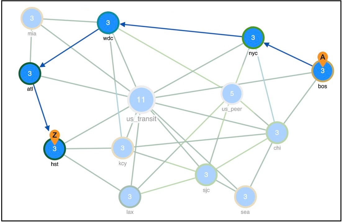
Click the demand from er1.bos to er1.hst.

The network plot shows this demand from "bos" to "hst" sites using a blue arrow to show the route, an A to show the source, and a Z to show the destination.

Figure 1. Demand route
Demand route
4.

Show the Service class column:

  1. Click the Show/hide table columns icon ().

  2. In the Search field, enter the word “service”. The Service class column name appears.

  3. Select the Service class check box

5.

Click the Service class column heading to sort demands by service class.

6.

Read the Traffic column values to determine how much traffic each demand is attempting to route.

7.

Determine the sum of the delays for all the interfaces on the longest path taken by each demand:

  1. In the Demands table, click the Maximum latency column heading and notice the values. For example, select a demand with maximum latency value of 23.

  2. Choose > Filter to interfaces. The Interfaces table opens and shows only the interfaces included in this demand.

  3. Click the Show/hide table columns icon () and select the check box for the Delay sim column.

    The Delay sim column appears on the Interfaces table.

  4. Notice that the sum of Delay sim values of all interfaces is equal to the maximum latency of the corresponding Demand. In this case, 23.

Clear the filter once you have completed the above steps.
8.

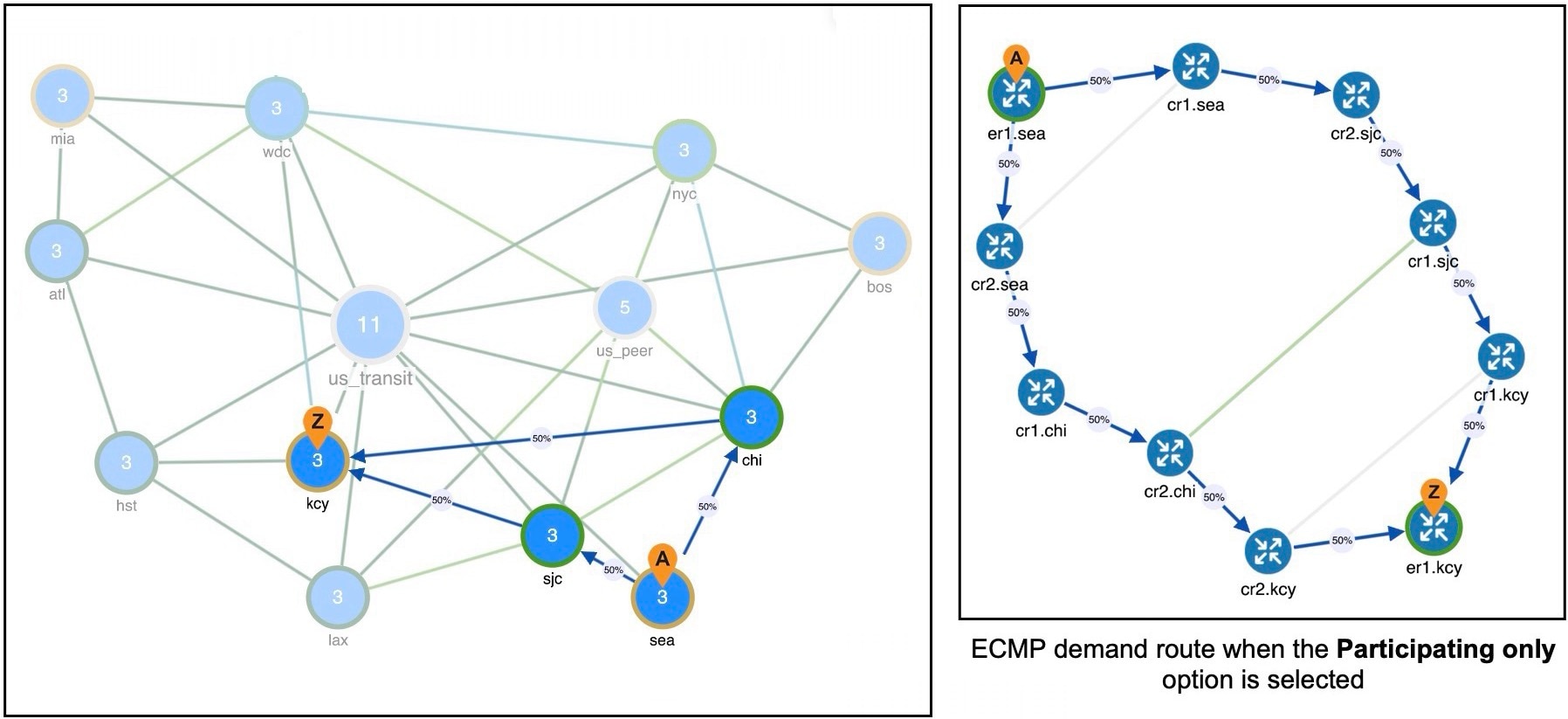
In the Demands table, notice the er1.sea to er1.key demand takes four equal-cost multipath (ECMP) routes. The number 50% indicates that 50% of the split demand is flowing through each of these circuits.

Select the Participating only check box in the network plot to view the details of the demand route. When you select this option, the network plot displays only the nodes associated with the demand route.

Figure 2. ECMP demand route
ECMP demand route

Modify demand traffic

You can modify demand traffic to determine the effects such changes in traffic have on the network. These modifications can be applied to regions or sites, or they can apply uniformly over the network. For example, you might increase the demand traffic to plan for future traffic growth by simulating an overall traffic growth trend. Another example might be to determine the network impact of an anticipated increase in sales of a particular service, such as video on demand.

You have numerous options for modifying demand traffic, all from the same window. The changes that you make apply to the selected demands for the current traffic level. You can modify demand traffic to either fixed values or to their relative values.


Modify fixed demand traffic

Use this task to modify fixed demand traffic.

Procedure

1.

Open the plan file (refer to Open plan files). It opens in the Network Design page.

2.

In the Network Summary panel on the right side, select one or more demands from the Demands table.

3.

Click Edit icon.

Note

If you are editing a single demand, you can also use the > Edit option under the Actions column.

4.

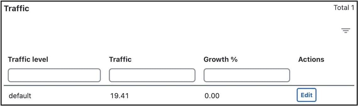
Under the Traffic section, click Edit under the Actions column.

Figure 3. Modify demand traffic
Modify demand traffic
5.

For each applicable traffic level, enter the desired amount of simulated traffic in the Traffic field and click Save.

6.

Click Save on the Edit Demand page.


Modify fixed or relative demand traffic

Use this task to modify the demand traffic to a fixed or relative value using the Modify demand traffic initializer.

Procedure

1.

Open the plan file (refer to Open plan files). It opens in the Network Design page.

2.

From the Traffic level drop-down list in the toolbar, select the traffic level you want the changes to apply to.

3.

From the toolbar, click Actions > Initializers > Modify demand traffic to open the Modify Demand Traffic page.

4.

Select the demands for which you want to modify the traffic. By default, all demands are selected. Deselect all and select the required demands.

5.

Click Next.

6.

Select one of the options listed in Demand traffic modification options and choose a relevant value.

7.

Submit your changes.


Demand traffic modification options

This table lists the available options for modifying demand traffic. Except for the percentage option, all values are in Mbps.
Table 1. Modify demand traffic options

Option

Description

Change traffic by __ %

Change traffic by a specified percentage. Positive percentages add to the traffic, and negative percentages subtract. For example, if the traffic were 1000 Mbps and you entered –10, the traffic would be reduced to 900 Mbps.

Add

  • Add __ Mbps in total, proportionally: Add a set amount of traffic spread over all demands in proportion to their current traffic. For example, if one demand had 1000 Mbps of traffic and the other had 2000 Mbps, and if you added 50 Mbps proportionally, one would have 1016.67 Mbps and the other would have 2033.33 Mbps.

  • Add __ Mbps in total, uniformly: Add a set amount of traffic uniformly to all the demands. For example, if one demand had 1000 Mbps of traffic and the other had 2000 Mbps, and if you added 50 Mbps uniformly, one would have 1025 Mbps and the other would have 2025 Mbps.

Set traffic to

  • Set traffic to __ Mbps each: Set traffic to a fixed value.

  • Set traffic to __ Mbps in total, proportionally: Set traffic to a specific value that is spread proportionally over all demands. For example, if one demand had 1000 Mbps of traffic and the other had 2000 Mbps, and if you set them to 4000 Mbps proportionally, one would have 1333.33 Mbps and the other would have 2666.67 Mbps.

  • Set traffic to __ Mbps in total, uniformly: Set a specified amount of traffic, in Mbps, uniformly to all the demands. For example, if one demand had 1000 Mbps of traffic and the other had 2000 Mbps, and if you set them to 4000 Mbps uniformly, they would both be 2000 Mbps.


Demand traffic modification example

This example details the effects of modifying the demand traffic of the selected demands by 50%.

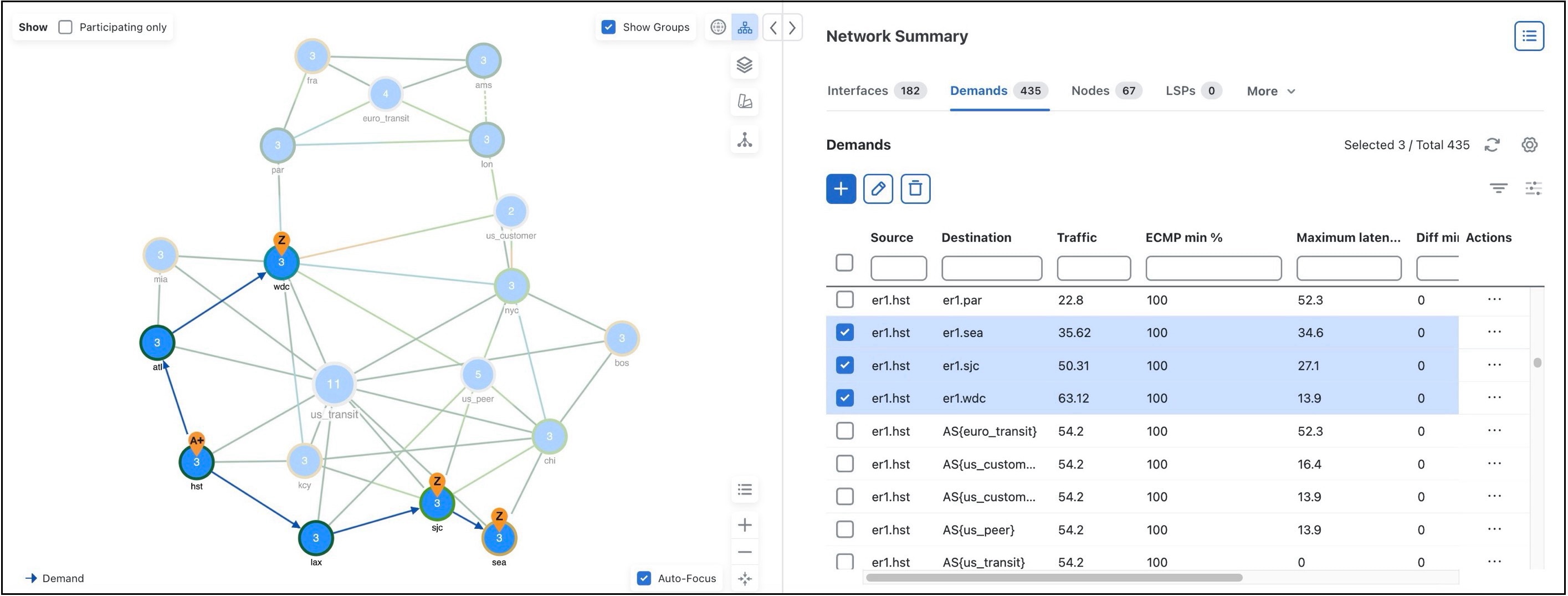
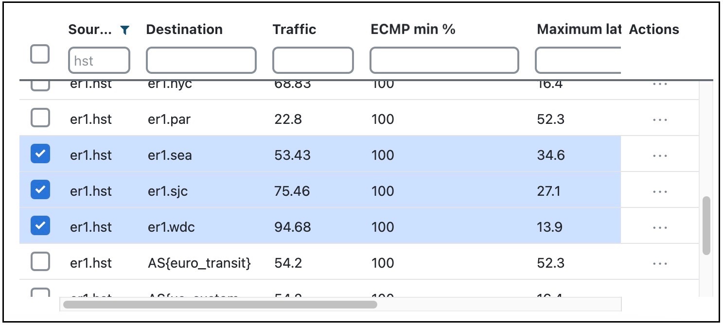
Note the values in the Traffic column for the demands: 35.62, 50.31, and 63.12 Mbps.

Figure 4. Demand traffic
Demand traffic

To increase the demand traffic by 50%, enter 50 in the Change traffic by ___ % field. Notice that the values in the Traffic column have increased by 50% to 53.43, 75.46, and 94.68 Mbps.

Figure 5. Demand traffic increased by 50%

Demand deduction

A demand deduction is a Cisco Crosswork Planning tool that

  • estimates demand traffic based on available measurements from network interfaces, queues, and LSPs, and

  • adjusts results for accuracy depending on the type and availability of measurements.

Network models contain traffic measurements on the discovered network. Traffic can be measured on interfaces, interface queues, and RSVP LSPs, as well as on general traffic flows, such as from LDP LSPs. You can use the Demand deduction tool to estimate demand traffic based on any of these measurements.

The accuracy and usefulness of the results depend on factors such as the amount and type of available measured traffic. For example, interface measurements are most often available, but LSP measurements might provide more information. The results also depend on the accuracy of the demand mesh and the routing model.

Typically, you only have interface traffic measurements. In this case, the individual demands estimated by Demand deduction are not necessarily accurate. However, aggregates of demands can be highly accurate. For example, you can predict the overall utilization after a failure, a topology change, or a metric change, even if the underlying demands individually are not reliable.

For more accuracy of individual demands, include point-to-point measurements, such as for RSVP LSPs or LDP flow measurements. Also, it is useful to combine different types of measurements together for use in Demand Deduction. Interface measurements are generally the most accurate measurements available, and if included in a Demand deduction, can correct for missing or inaccurate LSP or flow measurements.

Note that you can also use Demand deduction to set Traffic balance (%) values for external endpoint members that are set to a Deduce Traffic type.


Differences in measured and simulated traffic

Demand deduction relies on accurate topologies, demand meshes, and traffic measurements. These factors influence whether simulated traffic matches measured traffic and affect demand deduction accuracy.

You can see how close these values are by showing the Abs meas diff and Meas diff/cap (%) columns in the Interfaces table.

  • Abs meas diff: The difference between measured traffic (Traff meas) and simulated traffic (Traff sim).

  • Meas diff/cap (%): The absolute measured difference expressed as a percentage of capacity.

Causes for discrepancies between measured and simulated traffic

If these columns show large values, one of these situations likely exists:

  • Inaccurate measurements: Different measurements, for example of traffic through different interfaces, can be made at slightly different points in time. Fluctuations in traffic levels might take place between the times that measurements are being taken. This means that measurements could be inconsistent with one another. Usually, these inconsistencies are small and do not seriously affect the Demand deduction results.

  • Insufficient measurements: A network typically contains more demands than measurements. As a result, many solutions will fit the observed data well. Demand deduction chooses between possible solutions using knowledge of typical behavior of point-to-point traffic.

  • Incorrect network configurations: If the network topology is incorrect in the plan file, the simulated routes would naturally be incorrect and measurements would not be adequately interpreted.

  • Unbalanced ECMP: ECMP hashing can result in imperfect load balancing. Demand deduction, however, distributes traffic evenly across ECMPs.

  • Static routes: Cisco Crosswork Planning does not model static routes. If these are present, demands routes might be simulated incorrectly, leading to deduction errors.

  • Incomplete demand meshes: Demand meshes do not contain nodes even though traffic is routed between those nodes.

  • Inappropriate priorities: In the Demand Deduction window, you have the option to set the priority for calculations as 1 or 2. Cisco Crosswork Planning first uses the measurements identified as Priority 1 to calculate the demands. Therefore, if the priority settings do not match the consistency of the traffic measurements in the network, the simulated traffic measurements will be less than optimal.

Demand deduction warnings

Demand deduction displays warnings for misleading or undesirable results.

  • AS “(AS name)” contains both dynamic LSPs and interface traffic. Interface traffic in AS has been ignored.

    Routing of dynamic LSPs is non-deterministic. So it is not possible to make use of both measured interface traffic and measured dynamic LSP traffic for LSPs that may (or may not) traverse these interfaces. If the network contains an AS with both dynamic LSPs and interface traffic, this warning is issued. The interface traffic is not used.

  • Some interface measurements exceed capacities by as much as (percent).

    This warning is issued if a specified measurement exceeds the corresponding circuit capacity.


Strategies for minimizing differences between measured and simulated traffic

Demand deduction estimates demands that predict interface utilizations under incremental changes to the topology, including failures, metric changes, or design changes, such as adding a new express route. If only interface measurements are available, you might fine-tune the Demand deduction calculations to get better results, especially for site-to-site traffic.

To enhance the accuracy of Demand deduction results, consider these suggestions:
  • Include RSVP LSP or LDP measurements in the network discovery process.

  • Restrict demand meshes to exclude demands that are known to be zero.

    For example, if you know that core nodes do not source traffic, then exclude core nodes when creating the demand mesh.

  • Check the Nodes table to see if there is a node where the measured traffic going into it (Dest traff meas) and out of it (Source traff meas) are very different. Ensure these nodes are included in the demand mesh because they are either sources or destinations for traffic.

  • On the Demand Deduction page, set the most consistent measurements to a Priority 1. The most reliable measurements are usually interface measurements. Likewise, LSP measurements are end-to-end, and thus also generally highly reliable. You can set multiple measurements to priority 1.

    For example, if flow measurements are inconsistent and interface measurements are very consistent, set interface measurements to Priority 1 and the flow measurements to Priority 2.

  • If only a few measurements are available or if there are many inaccurate measurements, the tool sometimes estimates more traffic in a circuit than its capacity. To prevent this, on the Demand Deduction page, select the option to keep the interface utilization below 100%. This forces the resulting simulated calculations to be below the given percentage of circuit capacity.


Flow measurements for demand deduction

Besides node, interface, and LSP traffic measurements, Demand deduction allows more general flow measurements. These flow measurements can be flows from (or through) a specified node, to (or through) another node. You can also use combinations of these node-to-node flows. This measurement format can be used to enter, for example, peer-to-peer flow measurements, or traffic measurements obtained from LDP routing or from NetFlow.

Note

You can only view the Flows table if is already present in your plan file. You cannot create, edit, or delete the Flows in the UI.

Flow measurements are entered in the plan file in the <Flows> table. They appear in the UI in the Flows table. Table 1 lists some of the useful columns in the Flows table. The included traffic is defined by the From type and To type columns.

Table 2. Flows table columns

Column

Description

From

Specifies the source node.

From type

  • Source: Traffic originating at the From node is included in the flow.

  • Interior: Traffic is included that passes through the From node, entering that node from another node in the same AS

  • Border: Traffic is included that passes through the From node, entering that node from another node in a different AS.

To

Specifies the destination node.

To type

  • Dest: Traffic that is destined for the To node.

  • Interior: Traffic that passes through the To node to another node in the same AS.

  • Border: Traffic that passes through the To node to another node in a different AS.

Traff meas

Measured traffic used by Demand deduction in its calculations. If more than one node is included in either the From or To columns, this measurement is the sum of the traffic over all flows between individual pairs of From and To nodes.


Estimate demand traffic using demand deduction

The Demand deduction tool calculates demand traffic when traffic measurements are available.

The options available can significantly affect the calculations. For information on improving accuracy of results, refer to Strategies for minimizing differences between measured and simulated traffic. For information on setting up external endpoint members to be included in Demand deduction calculations, refer to Simulate Advanced Routing with External Endpoints.

Complete these steps to estimate the demand traffic using the Demand deduction tool.

Procedure

1.

Open the plan file (refer to Open plan files). It opens in the Network Design page.

2.

From the Traffic level drop-down list in the toolbar, select the traffic level on which you are creating simulated traffic. The measurements used come from this traffic level, and the simulated traffic for each demand is placed in this traffic level.

3.

From the toolbar, choose Actions > Tools > Demand deduction.

  1. (Optional) Modify the traffic measurements for one or more demands by clicking the Edit button in the Measurements (measurements / total) section. In the window that appears, you can modify measured traffic of interfaces.You can further change these measurements for a traffic level and interface queue.

    Another option in this window is to enter growth percents for use with the Create growth plans tool. For more information on creating growth plans, refer to Evaluate Impact of Traffic Growth.

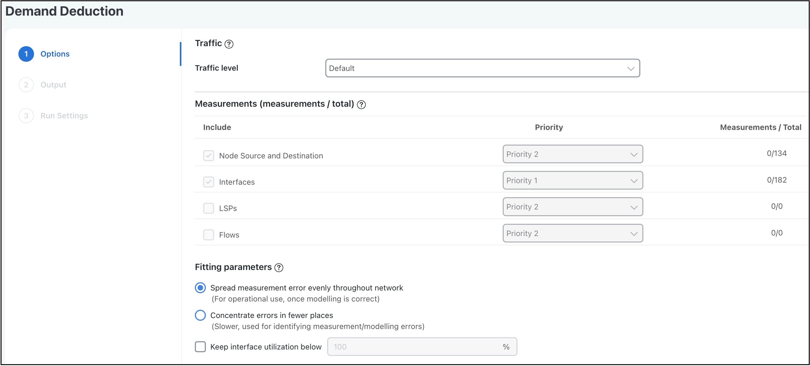
  2. Identify one or more types of measurements used in the calculations: Nodes (source and destination), Interfaces, LSPs, and Flows.

  3. For each type, set its priority. Select Priority 1 for high priority and Priority 2 for lower priority. You can have multiple measurements of the same priority. Like priorities are calculated simultaneously with equal consideration for the measurements.

    By default, all available measurements in the selected traffic set are used, and the interface measurements have priority over node, LSP, and flow measurements.

  4. Choose the required Fitting parameters.

  5. If you need to keep the traffic utilization below a different percentage than 100% (default), check the Keep interface utilization below __ % check box and enter a value.

  6. Click Next.

4.

Select the demands for use in constructing the demand calculations.

  • Use existing: Calculates demands using the existing demands only. This option is useful when simulating a pattern of demands that cannot be represented as a simple mesh between nodes. If you did not select one or more demands before opening this window, use this option.

  • Use selected: Calculates demands for the selected rows in the Demands table. This option is helpful when you want to recalculate some of the demands, for example, such as a VPN submesh.

5.

Determine whether to fix multicast demands. If selected, the multicast demands are fixed at their current traffic value.

6.

Determine whether to remove demands with zero traffic. The default is to remove them because Demand deduction typically estimates a significant percentage of the simulated traffic to be zero when a large number of point-to-point utilizations in a mesh are extremely small. Using this default can substantially improve simulation and optimization performance in large plans. Do not remove demands with zero traffic if all demand routes are of interest, irrespective of traffic. Click Next.

7.

On the Run Settings page, choose whether to execute the task now or schedule it for a later time. Choose one of these Execute options:

  • Now: Choose this option to execute the job immediately. The tool runs and changes are applied to the network model immediately. A summary report appears. You can access the report any time later using Actions > Reports > Generated reports option.

  • As a scheduled job: Choose this option to execute the task as an asynchronous job. Set these options:

    • Priority: Select the priority of the task.

    • Engine profiles: Select the engine profile as needed. This section lists all the available asynchronous engine profiles.

    • Schedule: Set the time at which you want to run the tool.

    The tool runs at the scheduled time using the selected engine profile. You can track the status of the job at any time using the Job Manager page (from the main menu, choose Job Manager). Once the job completes, import the output plan file into user space to visualize it. For more information, refer to Access output plan files from job manager.

    Note
    Ensure that you save the plan file before you schedule the job. Any unsaved changes in the plan file are not considered when you run the tool as a scheduled job.
8.

Submit your changes.

The Demand deduction tool calculates the simulated traffic and lists the results in a Demand Deduction report.

Demand deduction example

This example demonstrates results when using the Demand Deduction tool on a simple network.

Scenario overview

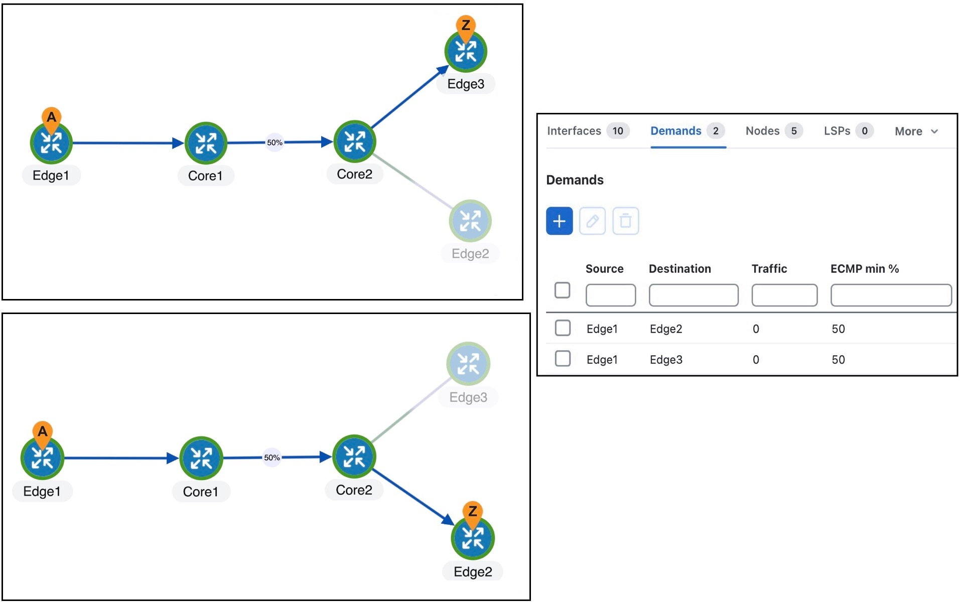
Network containing two demands and no demand traffic shows the routes of two demands in a network. These demands split between the two parallel core circuits due to an ECMP, and they have a common routing until the last hop. The Traffic column in the Demands table shows 0, as these demands do not contain any traffic yet.

Figure 6. Network containing two demands and no demand traffic
Network containing two demands and no demand traffic

Measured interface traffic

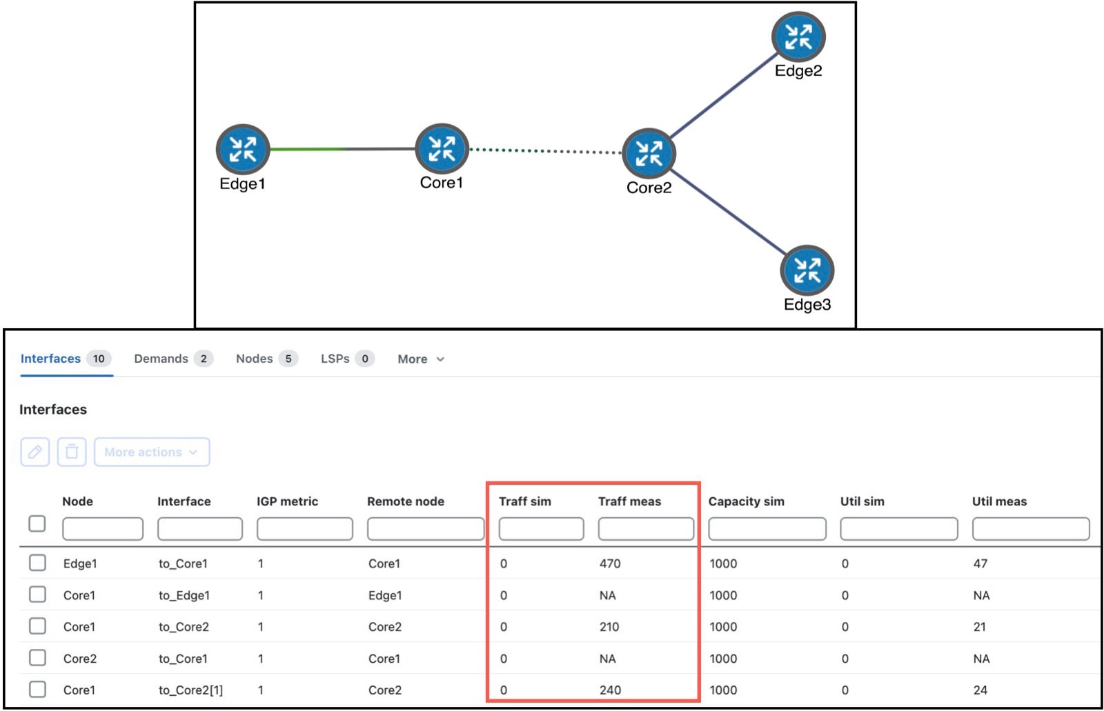
Measured traffic view and interfaces associated with the demands shows the Measured traffic view and the five interfaces associated with the two demands, three of which have measured traffic.

  • Edge1 to Core1 has 470 Mbps of measured traffic.

  • One Core1 to Core2 interface has 210 Mbps, and the other has 240 Mbps, making a total of 450 Mbps. This unequal split results from imperfect load balancing of the ECMP.

  • There is no traffic from Core2 to Edge2 or from Core2 to Edge3.

Figure 7. Measured traffic view and interfaces associated with the demands
Measured traffic view and interfaces associated with the demands

Demand deduction simulation

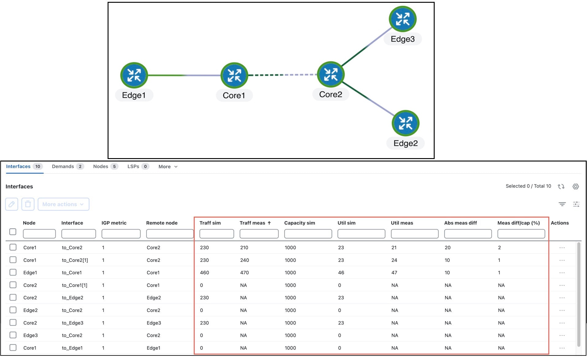
Upon running Demand deduction with its default options, the Simulated traffic view appears. Other than the measured interface traffic, there is no other information about the demand traffic. So, Demand deduction first splits the difference between the measured 470 Mbps of traffic (Edge1 to Core1) and the measured traffic of 450 Mbps (Core1 to Core2) to get an estimated total demand traffic of 460 Mbps. In the absence of any other information, it divides this 460 equally to give 230 Mbps of traffic to each demand (Simulated view showing demand traffic). In the Interfaces table, the Traff sim column now has values and the network plot shows simulated traffic percentages on all five interfaces associated with the demands.

  • Edge1 to Core1 has 460 Mbps of simulated traffic.

  • Both Core1 to Core2 interfaces have 230 Mbps.

  • Core2 to Edge2 and Core2 to Edge3 both have 230 Mbps.

    The Abs meas diff and Meas diff/cap (%) columns in the Interfaces table show mismatches between measured and simulated values.

  • Edge1 to Core1 has a difference of 10 Mbps, or 1%.

  • One Core1 to Core2 has a difference of 20 Mbps, or 2%, while the other has a difference of 10 Mbps, or 1%.

  • Neither the Core2 to Edge2, nor the Core2 to Edge3 interfaces have values because they had no measured traffic.

Figure 8. Simulated view showing demand traffic
Simulated view showing demand traffic

Alternate scenario

In this same example, if the Core2 to Edge2 interface had 50 Mbps traffic, the results would have been different. Because this interface is used only by the one demand, the measured 50 Mbps of traffic would be used as an estimate only for that one demand. Using the same logic as before, the demands should total to 460 Mbps, so the other demand is set to the difference, which is 410 Mbps.