- Overview
- User Interface
- Plan Objects
- Traffic Demand Modeling
- Simulation
- Simulation Analysis
- Traffic Forecasting
- IGP Simulation
- MPLS Simulation
- RSVP-TE Simulation
- Segment Routing Simulation
- Layer 1 Simulation
- Quality of Service Simulation
- BGP Simulation
- Advanced Routing with External Endpoints
- VPN Simulation
- Multicast Simulation
- Metric Optimization
- LSP Optimization
- RSVP-TE Optimization
- Explicit and Tactical RSVP-TE LSP Optimization
- Segment Routing Optimization
- Capacity Planning Optimization
- L1 Circuit Path Optimization
- Changeover
- Patch Files
- Reports
- Cost Modeling
- Plot Legend for Design Layouts
Cisco WAE Design 7.0.1 User Guide
Bias-Free Language
The documentation set for this product strives to use bias-free language. For the purposes of this documentation set, bias-free is defined as language that does not imply discrimination based on age, disability, gender, racial identity, ethnic identity, sexual orientation, socioeconomic status, and intersectionality. Exceptions may be present in the documentation due to language that is hardcoded in the user interfaces of the product software, language used based on RFP documentation, or language that is used by a referenced third-party product. Learn more about how Cisco is using Inclusive Language.
- Updated:
- May 4, 2017
Chapter: Plan Objects
Plan Objects
WAE Design networks consist of objects, such as nodes, sites, interfaces, circuits, SRLGs, ports, and port circuits. This chapter describes these basic objects and their relationships, as well as how to create, edit, and delete them.
Most objects are represented in the network plot, and all of them are represented in tables. Objects in the plot and in the associated tables have a set of properties that you can manage using a Properties dialog box. These object properties are represented by columns in the object’s table, or by entries in tables of related objects. For example, all circuits have a Capacity property.
WAE Design has both a Layer 3 (L3) view and a Layer 1 (L1) view, each containing objects.
Editing Objects Quick Reference
This table is a simplification of basic object editing capabilities. Not all tasks apply to all objects.
|
|
|
|
|
|---|---|---|---|
Understanding Nodes and Sites
Both node and site are WAE Design terminology.
- Node—A device in the network, which can be one of three types: physical, PSN (pseudonode), or virtual. The Type property distinguishes whether the node represents a real device or an abstraction, such as a single node representing a number of edge nodes connected in the same way to the network. A physical node is a Layer 3 device, or router. Physical and virtual nodes behave in the same way within WAE Design. A pseudo-node (PSN) is typically used to represent a Layer 2 device or a LAN.
Nodes can reside both inside and outside of sites. The external arrangement could be useful for small networks where routers are not geographically dispersed.
- Site—A collection of nodes and/or other sites that potentially form a hierarchy of sites. Any site that contains other sites is called the parent site.
Both nodes and sites have simulated traffic, while nodes also have measured traffic.
- Nodes are shown as rectangles. The border color is an indication of traffic sourced from and destined to the node.
- Sites are shown as squares. The border color indicates the traffic utilization of all the nodes and circuits inside the site, including all nested nodes and circuits.
Note that sites can contain both L3 nodes and L1 nodes. Empty sites appear in both views, as do sites containing both L3 and L1 nodes. Only sites containing L3 nodes appear in the L3 view, and only sites containing L1 nodes appear in the L1 view. To change these defaults, see the Cisco WAE Network Visualization Guide.
Parent Sites and Contained Objects
Unless a site is empty, there is a hierarchy of the sites and nodes that a site contains. A site can be both a parent and a child site. If a site contains another site, it is a parent site. Any nodes, sites, or circuits within a parent site are contained ( nested) objects. The contained nodes and sites are also called children. Often the child nodes and sites are geographically co-located. For example, a site might be a PoP where the routers reside.
- The site’s Parent Site property defines whether it is nested within another site. If it is empty, the site is not nested.
- In the network plot, the parent site shows all egress inter-site interfaces of all nodes contained within it, no matter how deeply the nodes are nested. Similarly, this is true for each child site plot within it.
- Selecting a site from the network plot does not select the sites or nodes under it.
- To filter to the sites or nodes contained within a site, right-click to access its “Filter to contained” menu. If you select “Direct,” WAE Design filters to only those objects contained immediately within it. If you select “All,” WAE Design filters to all objects contained within it, no matter how deeply they are nested.
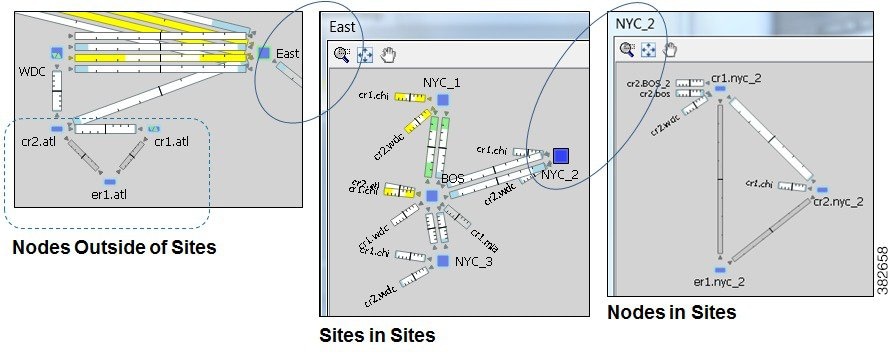
Figure 3-1 shows an example of nodes outside of sites (atl nodes), sites containing other sites (the East site contains three NYC sites and one BOS site), and nodes within a site (NYC_2 site contains three nyc nodes). While this figure only shows one of the child site plots, if you were to expand all nested sites with the East site, you would find more nested child sites and nodes. As you can see in the network plot, the East site has 10 egress interfaces extending from it, some of which are within nested sites.
Figure 3-1 Example of Node and Site Relationships
Deleting Sites
Selecting a site from the network plot does not select the sites or nodes under it except when deleting the site. In this case, all objects within a site are selected for deletion. However, in the confirmation that appears, you have the option to keep the contained sites and nodes. If you do, then the objects that are contained directly within it are moved to be on the same level as the site that is removed. The other, more deeply nested objects maintain their parent relationships.
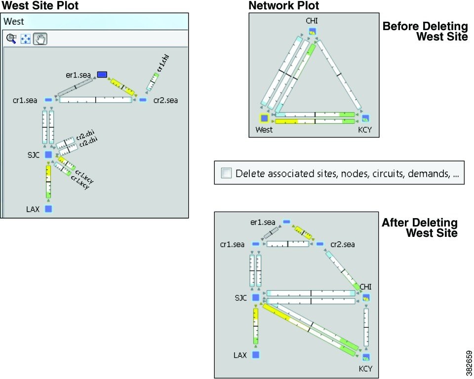
Figure 3-2 shows a West site plot directly containing two sites (SJC and LAX) and three nodes. This parent West site resides in the network plot. Both SJC and LAX contain two sites each. By deleting the West site plot, but retaining its children, both SJC and LAX move to the network plot level, as do the three sea nodes. The sites within SJC and LAX remain as children sites to their respective parent sites.
Figure 3-2 Example Site Deletion
PSN Nodes
WAE Design plan files can contain nodes of with a Type property of “psn.” These nodes represent pseudonodes (PSNs), which are used to model LANs or switches that connect together more than two routers. They are used in two situations: for IGP modeling and BGP peer modeling.
In an IGP network, a LAN interconnecting multiple routers is represented by a PSN node, with circuits connected to each of the nodes representing the interconnected routers. Both OSPF and IS-IS have a built-in system whereby one of the routers on that LAN is the designated router (DR) for OSPF or the designated intermediate system (DIS) for IS-IS. The PSN node is named after this designated router. WAE creates nodes with a property Type of psn automatically during IGP discovery.
When BGP peers are discovered, WAE might find that a router is connected to multiple peers using a single interface. This is typical at switched Internet Exchange Points (IXPs). WAE then creates a node with a property Type of psn, and connects all the peers to it, each on a different interface.
Following are a few points to consider when working with nodes that have psn as a Type property.
- Two PSNs cannot be connected by a circuit.
- If a PSN node is created by WAE, “psn” is prepended to the designated router’s node name.
- When creating demand meshes, WAE Design does not create demands with nodes of Type psn as sources or destinations. This is possible in manual demand creation, but not recommended. WAE Design sets the IGP metric for all egress interfaces from a node of Type psn to zero. This ensures that the presence of a PSN in a route does not add to the IGP length of the path.
Creating Nodes and Sites
Creating Nodes
To create a node, either choose Insert > Node, or right-click in an empty plot area and choose New > Node. Following are some of the frequently used fields:
- Name—Required unique name for the node.
- IP Address—Often the loopback address used for the router ID.
- Site—Name of the site in which the node exists. If left empty, the node resides in the network plot. This offers a convenient way to create a site while creating the node, move nodes from one site to another, or remove nodes from a site so it stands alone in the network plot.
- AS—Name of the AS in which this node resides, which identifies its routing policy. This can be left empty if no BGP is being simulated.
- BGP ID—IP address that is used for BGP.
- Function—Identifies whether this is a core or edge node.
- Type—The node type, which is physical, PSN, or virtual. Because a PSN node represents a Layer 2 device or a LAN, interfaces on a PSN must all have their IGP metrics set to zero, and two PSN nodes cannot be directly connected to one another. If you change a node type to PSN, WAE Design automatically changes the IGP metrics on its associated interfaces to zero.
- Longitude and Latitude—Geographic location of the node within the network plot. These values are relevant when using geographic backgrounds.
- X and Y—Location of the node within the network plot. These values are relevant when using schematic backgrounds.
Creating Sites
To create a site, either choose Insert > Site, or right-click in an empty plot area and choose New > Site. Following are some of the frequently used fields:
- Name—Required unique name for the site.
- Display Name—Site name that appears in the plot. If this field is empty, the Name entry is used.
- Parent Site—The site that immediately contains this site. If empty, the site is not contained within another one.
- Location—To automatically place a site in its correct geographic location and update the Longitude and Latitude fields, enter the airport code and press Enter. To select from a list of cities worldwide, press Alt-Enter.
- Longitude and Latitude—Geographic location of the site within the network plot. These values are relevant when using geographic backgrounds.
- Screen X and Y—Location of the site within the network plot. These values are relevant when using schematic backgrounds.
Duplicating Nodes
Duplicating a node creates an identical node and duplicates the connectivity of that node by creating new, identical circuits containing the same amount of traffic. By default, each demand and each LSP that uses the node as a source or destination is also duplicated. The newly created node is sequentially named the same. For example, if you duplicate a node named “chi,” WAE Design creates a chi[1] node. If you duplicate it again, a chi[2] node is created.
Step 1![]() Use one of these methods to open the Duplicate Node dialog box:
Use one of these methods to open the Duplicate Node dialog box:
Step 2![]() Select whether to duplicate demands and LSPs, and then click OK.
Select whether to duplicate demands and LSPs, and then click OK.
Duplicating Sites
Duplicating a site creates an identical site, including the nodes within it and its connectivity. The default site name and display name are the same as the copied site plus a sequential number. For example, duplicating OKC creates OKC[1]. However, you have the option to change both the site name and the display name. The nodes that are created are likewise sequentially renamed. To change a duplicated node name, open the node’s Properties dialog box.
You cannot duplicate a site that contains other sites.
Step 1![]() Use one of these methods to open the Duplicate Site dialog box:
Use one of these methods to open the Duplicate Site dialog box:
Step 2![]() If desired, rename the new site or display name, and click OK.
If desired, rename the new site or display name, and click OK.
Merging Nodes
Real network topologies often have a number of nodes, typically edge nodes, connected to the network in the same way. For example, they might all be connected to the same core node or pair of core nodes. For planning and design of the network core, it is often desirable to merge these physical nodes into a single virtual node, which simplifies the plan and accelerates the calculations and simulations performed. Note that merging nodes changes the plan itself, not just the visual representation.
The name of a newly merged node can be based on the site name, selected node name (base node), or have a new user-specified name. The node merge effects are as follows:
- Reattach circuits from other nodes to the base node.
- Move demands to or from other nodes to the base node.
- Move LSPs to or from other nodes to the base node.
- Set base node traffic measurements to the sum of measurements of the selected nodes.
- Delete other nodes.
Step 1![]() Select multiple nodes. If you do not select nodes, WAE Design merges all nodes.
Select multiple nodes. If you do not select nodes, WAE Design merges all nodes.
Step 2![]() Choose Initializers > Merge Nodes, or right-click one of the nodes and choose Merge.
Choose Initializers > Merge Nodes, or right-click one of the nodes and choose Merge.
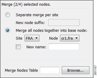
Step 3![]() Select whether to merge the nodes per site or merge them into one node.
Select whether to merge the nodes per site or merge them into one node.
- Separate merge per site—Merges nodes on a per-site basis. For example, if you selected all nodes in the plan, the result would be one merged node per site. If you do not specify a new suffix, the default name is the same as the site.
- Merge all nodes together into base node—Merges all nodes selected into one node. For example, if you selected two nodes in one site and three nodes in another, the result would be a single node in the site and node combination selected as the base node.
If you do not specify a new name, the default is to use the name of the base node.
Trimming Nodes and Moving Their Traffic
A plan file created through WAE discovery often has more edge nodes in the plot than you are interested in viewing or simulating. These might be nodes that forward very little traffic or are singly connected to the core. However, you can reduce such a network model in WAE Design for simplicity and performance improvements by trimming (removing) these nodes. This process also removes all associated circuits, demands, and external endpoints.
Note that you can either select nodes to trim or you can choose to trim all nodes except those that are selected.
Typically, plan files are trimmed before demands are created. However, you can optionally trim demands in a plan file. This moves a demand that is sourced on a trimmed node to the first hop on the demand path in the remaining network. Likewise, a destination to a trimmed node is moved to the last hop of the demand path in the remaining network. If two or more demands in the same service class are trimmed so that their resulting source and destination nodes are equal, these demands are aggregated into one demand with their traffic summed. Demands split by ECMPs are converted into multiple demands, each with traffic divided proportionally to the ECMP split.
Trimming a node is not the same as deleting a node. When you trim a node, the measured traffic carried through that node is transferred to the nodes that remain so that the overall traffic in the network remains unchanged. If the node is deleted, this traffic is discarded. Only measured traffic is preserved in this way.
Note that multicast demands are removed, and cannot be trimmed.
Example: Edge node E is singly connected to node C in the core. When E is trimmed, the measured traffic on the interface from E to C is added to the total source traffic on node C. The measured traffic on the interface from C to E is added to the total destination traffic on node C. By default, demands to and from node E are removed.
Example: A demand source is node A, and destination is node E, and is routed through nodes A-B-C-D-E. If nodes A and E are trimmed and if you select the option to trim demands, then the new route for the demand is B-C-D.
Step 1![]() (Optional) If you want to trim the traffic of nodes under a specific utilization, sort one of the Traffic columns to find the lowest to highest utilization. Alternatively, use the Nodes table filter to search for traffic of a certain level using, for example, the less than operator (<).
(Optional) If you want to trim the traffic of nodes under a specific utilization, sort one of the Traffic columns to find the lowest to highest utilization. Alternatively, use the Nodes table filter to search for traffic of a certain level using, for example, the less than operator (<).
Step 2![]() Select one or more nodes that you either want to trim or that you want to preserve while trimming nodes.
Select one or more nodes that you either want to trim or that you want to preserve while trimming nodes.
Step 3![]() Right-click and choose Trim.
Right-click and choose Trim.
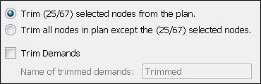
Step 4![]() Select whether to trim the nodes or to keep the nodes and trim those that are unselected.
Select whether to trim the nodes or to keep the nodes and trim those that are unselected.
Step 5![]() (Optional) Select the option to trim demands.
(Optional) Select the option to trim demands.
By default, the moved demands are named “Trimmed,” though you can enter a different name.
Circuits and Interfaces
In WAE Design, an interface is a either an individual logical interface or a LAG logical interface. If there is a one-to-one mapping between a logical and physical interface, then the interface contains both Layer 3 properties (for example, Metric) and physical properties (for example, Capacity). If there is a one-to-many mapping between logical and physical interfaces, then the interface is the logical LAG and the ports are included in the plan file as the physical ports in the LAG. For more information on ports and port circuits, see Ports, Port Circuits, and LAGs.
Each circuit connects a pair of interfaces on two different nodes. Therefore, an interface always has an associated circuit. Both the interface Properties dialog box and the circuit Properties dialog box let you simultaneously edit properties for the pair of interfaces and the circuit.
Interfaces have both measured and simulated traffic. The traffic that appears in the Circuits table is the higher of the traffic in the two interfaces.
Layer 1 Relationships
Each circuit can be connected directly to an L1 circuit. To make this connection, select the circuit, and either select or create the L1 circuit from the Advanced tab. An L3 circuit can be associated to multiple port circuits, and each port circuit can be associated with a different L1 circuit. Thus, L3 circuits can be associated indirectly with multiple L1 circuits. For more information, see Ports, Port Circuits, and LAGs and Layer 1 Simulation .
The Latency and Distance Initializer uses mapped L1 circuit delays to calculate L3 circuit delays. If L1 circuits are not mapped to the L3 circuits, the node Longitude and Latitude properties are used in the calculation. For information, see Simulation .
Creating Circuits and Interfaces
To create a circuit, choose Insert > Circuit, or right-click in an empty plot area and choose New > Circuit.
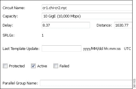
As a result of creating a circuit, two interfaces are also created.
- Capacity—The amount of total traffic this circuit can carry. The drop-down list has a selection of the most widely used capacities.
- SRLGs—If you want this circuit to belong to an SRLG, select it from this list or create a new one by clicking Edit. See Creating SRLGs for Circuits Only.
- Parallel Group Name—To include this circuit in a new or existing parallel grouping, enter its name. To visually combine these parallel groups in the network plot, see the Cisco WAE Network Visualization Guide.
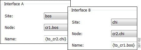
- Interface A and B—You must specify two interfaces that are connected by the circuit.
Duplicating Circuits
Duplicating a circuit has the following effect on the new circuit and its interfaces:
- Duplicates the circuit itself and all its properties, including the circuit name.
- As a result, it duplicates both associated interfaces and renames them by adding an incremental numeric suffix to the original names, such as [1]. All other interface properties are copied to the new interfaces.

Step 1![]() Select one or more circuits to duplicate.
Select one or more circuits to duplicate.
Step 2![]() Right-click one of these circuits and choose Duplicate.
Right-click one of these circuits and choose Duplicate.
Step 3![]() Enter the number of new circuits you want to create for each selected circuit. For example, if you selected two circuits and you enter 3, each of the selected circuits has three new parallel circuits, for a total of six new circuits.
Enter the number of new circuits you want to create for each selected circuit. For example, if you selected two circuits and you enter 3, each of the selected circuits has three new parallel circuits, for a total of six new circuits.
Step 4![]() To duplicate L1 circuits that are mapped to selected L3 circuits, check Duplicate mapped L1 Circuits.
To duplicate L1 circuits that are mapped to selected L3 circuits, check Duplicate mapped L1 Circuits.
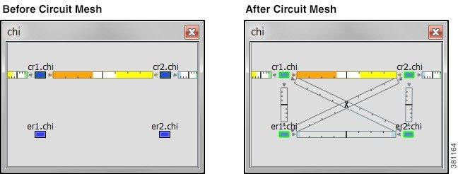
Creating a Circuit Mesh Between Nodes
To create a mesh of circuits between multiple nodes, follow these steps. Figure 3-3 shows an example circuit mesh created between all the nodes within a site.
Step 1![]() Select multiple nodes that you want to interconnect.
Select multiple nodes that you want to interconnect.
Step 2![]() Right-click the interface you want to duplicate and choose Duplicate Between Selected Nodes.
Right-click the interface you want to duplicate and choose Duplicate Between Selected Nodes.
Figure 3-3 Example Circuit Mesh
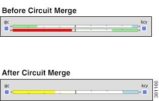
Merging Circuits
You can simplify the plan by merging circuits that have the same source and destination endpoints (nodes). This capability is useful, for example, in long-term capacity planning where multiple parallel circuits can be ignored and only the site-to-site connections are of interest.
Merging circuits changes the plan itself, not just the visual representation. (To change only the visual representation, see the Cisco WAE Network Visualization Guide.)
The circuit merge effects are as follows:
- Set base circuit capacity to the sum of capacities.
- Set base circuit metric to minimum of metrics.
- Set base traffic measurements to the sum of measurements.
- Delete other circuits.
Step 1![]() Select multiple circuits that have the same source and destination endpoints.
Select multiple circuits that have the same source and destination endpoints.
Step 2![]() Choose Initializers > Merge Circuits, or right-click one of the circuits and choose Merge.
Choose Initializers > Merge Circuits, or right-click one of the circuits and choose Merge.
Step 3![]() The name of a newly merged circuit is based on the selected circuit. If you want to base the name on a different circuit, select it from the Base Circuit list.
The name of a newly merged circuit is based on the selected circuit. If you want to base the name on a different circuit, select it from the Base Circuit list.
SRLGs
An SRLG is a group of objects that might all fail due to a common cause. For example, an SRLG could contain all the circuits whose interfaces belong to a common line card.
Creating SRLGs
Step 1![]() To open the SRLG dialog box, do one of the following:
To open the SRLG dialog box, do one of the following:
Step 2![]() Enter the SRLG name, or keep the sequentially named default names (SRLG1, SRLG2, and so on).
Enter the SRLG name, or keep the sequentially named default names (SRLG1, SRLG2, and so on).
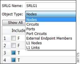
Step 3![]() From the Object Type drop-down list, choose the type of object that you want to include in the SRLG.
From the Object Type drop-down list, choose the type of object that you want to include in the SRLG.
Step 4![]() For each that object you want to include in the SRLG, check the F (false) check box to toggle it to T (true).
For each that object you want to include in the SRLG, check the F (false) check box to toggle it to T (true).
Step 5![]() Repeat Step 3 and Step 4 for each object included, and then click OK.
Repeat Step 3 and Step 4 for each object included, and then click OK.
Creating SRLGs for Circuits Only
Step 1![]() Open the Circuits Properties dialog box.
Open the Circuits Properties dialog box.
- If you are creating SRLGs for selected circuits, select one or more circuits. Then double-click one of them. This is a very quick method of adding numerous circuits to an SRLG.
- If you are creating a new circuit, right-click in an empty plot area and choose New > Circuit. For more information, see Creating Circuits and Interfaces.
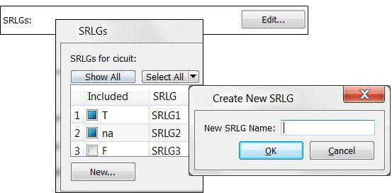
Step 2![]() Click the Edit button associated with the SRLG field.
Click the Edit button associated with the SRLG field.
Step 3![]() Associate the circuits with one or more existing SRLGs, or create a new SRLG.
Associate the circuits with one or more existing SRLGs, or create a new SRLG.
Step 4![]() Click OK in the SRLG dialog box to save the changes, and click OK again in the Properties dialog box.
Click OK in the SRLG dialog box to save the changes, and click OK again in the Properties dialog box.
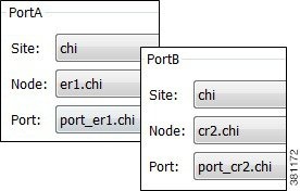
Ports, Port Circuits, and LAGs
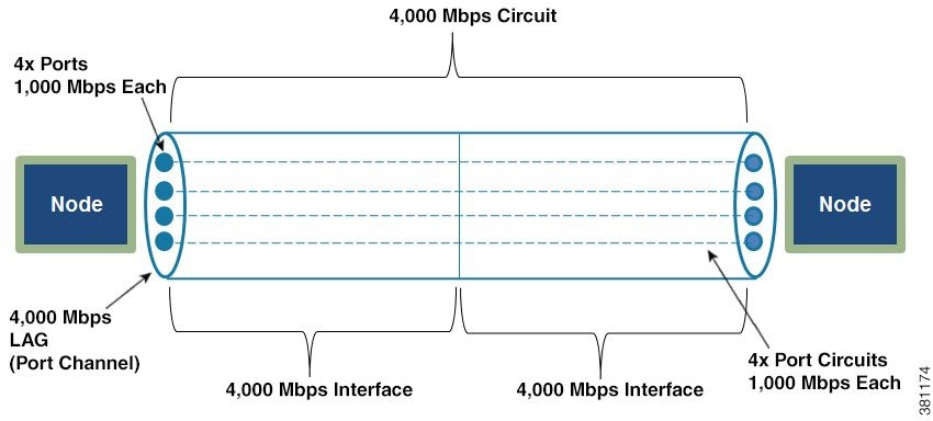
In WAE Design, a port is a physical interface. You can model link aggregation groups (LAGs) and port channels using WAE Design port and port circuits (Figure 3-4).
A LAG is a group of physical ports that are bundled into a single logical interface. A LAG is also known as bundling or trunking.
By default, each logical interface listed in the Interfaces table corresponds to a single physical port, and these ports need not be explicitly modeled. The exception is when the logical interface is a LAG, which bundles more than one physical port. In this case, the physical ports are listed in the Ports table.
A port circuit is a connection between two ports. However, ports are not required to be connected to other ports by port circuits.
Port circuits can be associated with L1 circuits, and ports can be connected to L1 nodes. The port circuit’s Delay Sim value is copied from the associated L1 circuit’s Delay Sim property. Otherwise, the Delay Sim value is set to 0. For information on L3 Delay and Delay Sim calculations, see Simulation . For information on L1 Delay and Delay Sim calculations, see Layer 1 Simulation .
Figure 3-4 Ports, Port Circuits, and LAGs
Creating Ports
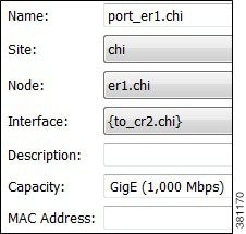
To create a port, either choose Insert > Port, or right-click in an empty plot area and choose New > Port. Following are some of the frequently used fields:
- Site and Node—Site and node on which this port exists.
- Interface—Logical interface to which this port is mapped. This must be defined to create port circuits using this port.
- Capacity—The amount of total traffic this port can carry. The drop-down list has a selection of the most widely used capacities.
Layer 1 Relationships
Each port can be connected to an L1 node or to both an L1 node and an L1 port. Creating these connections populates the L1 Node and L1 port columns in the Ports table. If this port belongs to a port circuit, the Remote L1 Node and Remote L1 Port columns are updated, as applicable.
To connect the port to an L1 node or L1 port, select the Layer 1 tab. Then select the site (if applicable), the L1 node, and the L1 port to which the port is connected. For more information on Layer 1, see Layer 1 Simulation .
Creating Port Circuits
A port circuit specifies a pair of connected ports.
- Both of the ports must exist and be mapped to interfaces that are connected by a circuit.
- When selecting the two ports for the port circuit, note that if one is assigned to an interface, the other must be assigned to the remote interface on the same circuit.
To create ports and map them to their interfaces, see Creating Ports.
To create a port circuit, either choose Insert > Port Circuit, or right-click in an empty plot area and choose New > Port Circuit. The site, node, and port are all required fields.
- Site and Node—Site and node on which the port exists.
- Port—Name of the port.
- Capacity—The amount of total traffic this port circuit can carry. The drop-down list has a selection of the most widely used capacities.
Each port circuit can be indirectly associated with an L1 circuit via direct mappings of L1 ports to L3 ports. For more information on Layer 1, see Layer 1 Simulation .
Creating LAGs
To make one of the existing interfaces into a LAG by assigning ports to it, follow these steps. If the interface does not contain ports, you must first create them (see Creating Ports).
Step 1![]() From the Ports table, select all ports that belong to the LAG. You can quickly do this by filtering to their common interface.
From the Ports table, select all ports that belong to the LAG. You can quickly do this by filtering to their common interface.
Step 2![]() Double-click one of the ports to open the Properties dialog box.
Double-click one of the ports to open the Properties dialog box.
a.![]() Select the interface that contains these ports.
Select the interface that contains these ports.
Setting LAG Simulation Properties
Each interface is considered to be a LAG (port channel). You can configure LAG properties so that if it loses too much capacity due to non-operational ports, the entire LAG is taken down.
Step 1![]() Double-click an interface or circuit; the Properties dialog box opens.
Double-click an interface or circuit; the Properties dialog box opens.
Step 2![]() Click the Advanced tab.
Click the Advanced tab.
Step 3![]() In the Port Channel area, set one or both of the following parameters for one or both interfaces on the circuit:
In the Port Channel area, set one or both of the following parameters for one or both interfaces on the circuit:
a.![]() In the Min Number of Ports field, enter the minimum number of ports that must be active and operating for the LAG circuit to be up.
In the Min Number of Ports field, enter the minimum number of ports that must be active and operating for the LAG circuit to be up.
b.![]() In the Min Capacity field, enter the minimum capacity that must be available for the LAG circuit to be up.
In the Min Capacity field, enter the minimum capacity that must be available for the LAG circuit to be up.
Editing Object Properties
Most objects in the plot and in the associated tables have a set of properties that you can manage using a Properties dialog box. These are the properties that WAE Design uses to define and simulate an object.
To change the properties of individual objects, do one of the following to open the Properties dialog box:
- Right-click one or more objects from the network plot or a table and choose Properties.
- Double-click one or more objects from the network plot or table. (The exception is that double-clicking a site from the plot opens a site plot.)
The Properties dialog box always lists how many objects were selected before opening the dialog box. For example, if the plan file includes 500 interfaces, and you have 342 of them selected, the notation is 342/500.
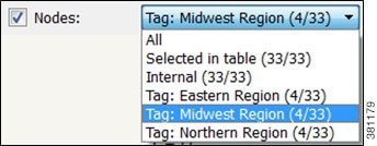
Tags
Many objects can be tagged as a way to group them for subsequent processing. Once created, tags appear as options in dialog boxes, enabling you to select and act upon all objects with a given tag name. Thus, tags provide a very flexible way to group interfaces, demands, nodes, LSPs, sites, and ASes that are not easily selected using standard attributes. For example, when using LSP paths you might want to tag selected paths to make it easier to assign or change their path affinities.
Adding tags to a parent site does not add tags to its children sites and nodes.
Adding Tags
Step 1![]() Right-click one or more objects and choose Properties.
Right-click one or more objects and choose Properties.
Step 2![]() Click the Tags tab and then New Tag.
Click the Tags tab and then New Tag.
Step 3![]() Enter a name that identifies the objects you are tagging (for example, Midwest Region), then click OK.
Enter a name that identifies the objects you are tagging (for example, Midwest Region), then click OK.
Enabling and Disabling Tags
Step 1![]() Right-click one or more objects and choose Properties.
Right-click one or more objects and choose Properties.
Step 2![]() Click the Tags tab; a list of available tags opens.
Click the Tags tab; a list of available tags opens.
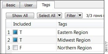
Step 3![]() Toggle the tags to enable (T is true) or disable (F is false).
Toggle the tags to enable (T is true) or disable (F is false).
 Feedback