Cisco WAE Design 7.0.1 User Guide

Disjoint Routing Selection

Only existing LSP paths are rerouted. New LSP paths are not created.

• Explicit hops are modified or created for RSVP LSPs.
• Segment list hops are modified or created for SR LSPs. The final hop is either a node hop or interface whose remote node is the destination of the LSP.

Segment lists are created only for LSP paths, and only LSP path segment lists are updated. If a segment list is associated with an LSP (rather than an LSP path), that LSP segment list is removed.

Routing options include:

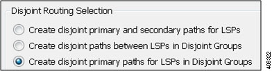
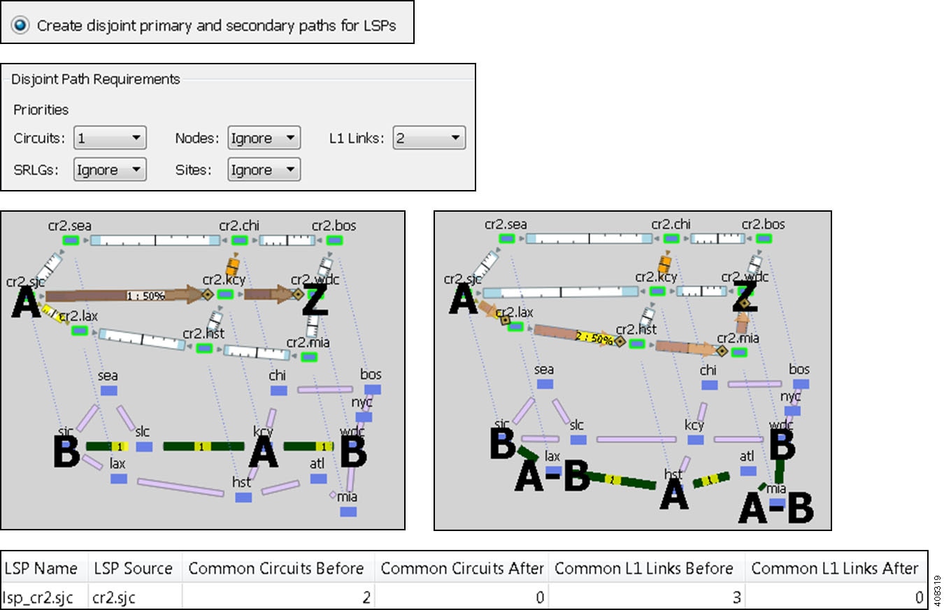
• Create disjoint primary and secondary paths for LSPs—For all LSPs, whether they are in a disjoint group or not, route all LSP paths so that they are disjoint from all other paths belonging to that LSP. This disjointness extends beyond primary and secondary paths to include all other path options (for example, tertiary).
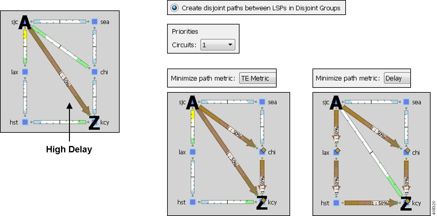
• Create disjoint paths between LSPs in disjoint groups—For all LSPs that are in disjoint groups, route all LSP paths so that they are disjoint from all other paths belonging to LSPs in that disjoint group. This disjointness extends beyond primary and secondary paths to include all other path options (for example, tertiary).

Example: All LSPs in disjoint group East are rerouted to be disjoint from each other. All LSPs in disjoint group Southeast are rerouted to be disjoint from each other. However, LSP paths in the East group are not rerouted to be disjoint from those in the Southeast group.

• Create disjoint primary paths for LSPs in disjoint groups—For all LSPs that are in disjoint groups, reroute only their primary paths so that they are disjoint from each other.

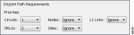
Disjoint Path Requirements

The disjoint path requirements identify the priority for creating disjointness across a path. Disjointness priorities 1, 2, 3, and Ignore are available for circuits, SRLGs, nodes, sites, and L1 links. The tool tries to create disjointness for all objects that have a priority set other than Ignore. If full disjointness cannot be achieved, the tool prioritizes disjointness based on these values.

Example: Circuits have a priority of 1, SRLGs have a priority of 2, and the other objects are ignored. If the tool cannot achieve full disjointness across both circuits and SRLGs, it prioritizes the disjointness of circuits over SRLGs.

Example

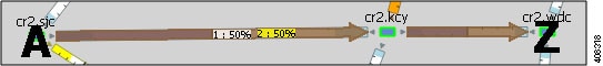
This example shows how disjoint routes can be created for primary and secondary RSVP LSP paths, and how those routes differ, depending on the path requirements set.

The LSP has a primary and secondary LSP paths that use the same route from cr2.sjc to cr2.wdc. The LSP is not a member of a disjoint group.

In both Figure 19-1 and Figure 19-2, the option is selected to create disjoint primary and secondary paths for LSPs. However, they show different secondary path routes.

• Figure 19-1 shows explicit interface hops set for the secondary LSP path that force it to take a different (northern) route from cr2.sjc to cr2.wdc. Because the disjoint path requirement is only circuits, the primary and secondary paths route across different circuits, as indicated in the resulting report. However, they share a common L1 link between slc and kcy.
• Figure 19-2 is based on setting circuits as the first priority for disjoint requirement and L1 links as the second priority. The result is a different set of explicit hops for the secondary LSP path, routing it through southern disjoint circuits that are mapped to different L1 links. The resulting report shows there are no longer any common L1 links.

Figure 19-1 Primary and Secondary Paths Based on Disjoint Circuit Requirements

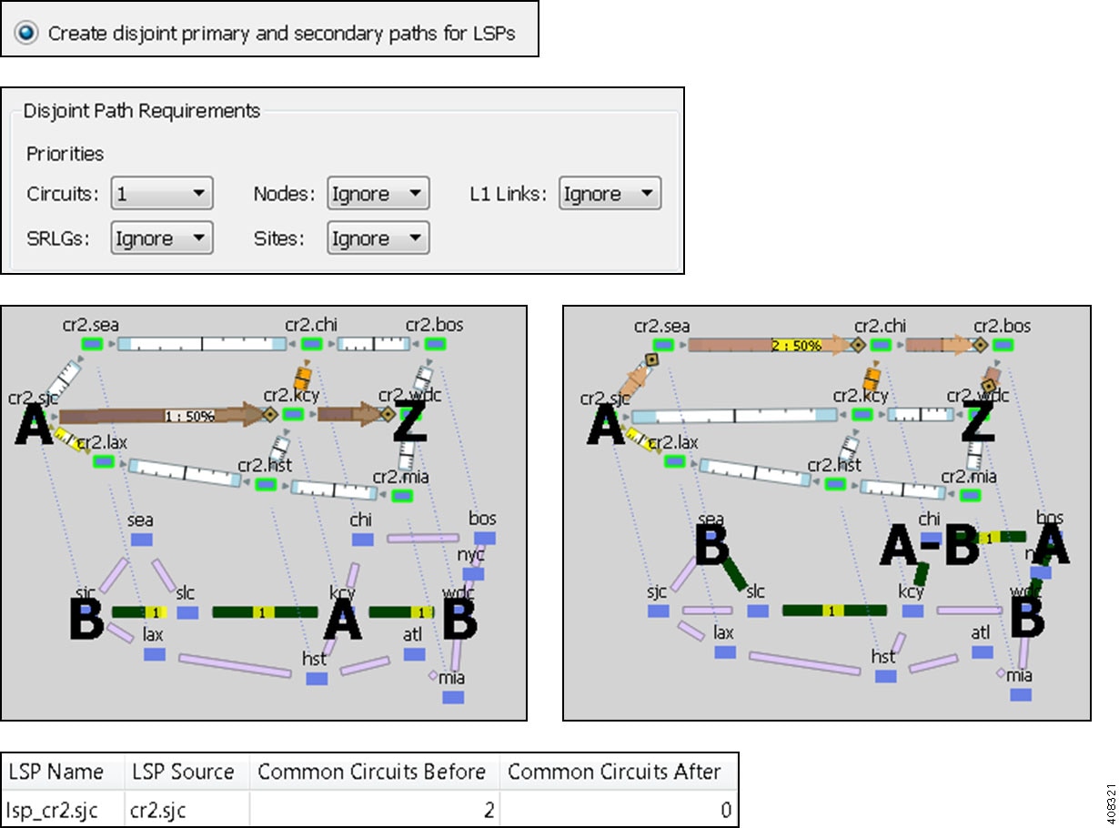
Figure 19-2 Primary and Secondary Paths Based on Disjoint Circuit and L1 Link Requirements

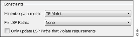
Constraints

• Minimize path metric—Paths are optimized to minimize the sum of the metrics along the path with respect to delay, TE, or IGP metrics. All of these properties are configurable from an interface Properties dialog box, and delays can also be set in a circuit Properties dialog box.
• Fix LSP Paths—Selected or tagged LSP paths are not rerouted. This constraint is useful when you have previously optimized specific LSPs within the network and want to maintain their routes.
• Only update LSP Paths that violate requirements—Paths are modified only if they violate the requirements specified in the Disjoint Path Requirements area of the dialog box.

Example

This example shows how disjoint routes can be optimized for two SR LSPs using the same source (sjc) and destination (kcy).

• Both LSPs belong to the same disjoint group, and both LSPs have an LSP path.
• The circuit between sjc and kcy has significantly higher delay than the other circuits.
• The only disjoint path requirement selected is circuits.
• Figure 19-3 shows the following:

– Before using the LSP Disjoint Path Optimization tool, both LSP paths use the same route. There are no segment list hops.

– By selecting the option to create disjoint paths between LSPs in the same disjoint group and using the TE metric for the shortest path calculation, two disjoint LSP path routes are created. Both have a segment list node hop on the destination node. One has an additional segment list node hop on chi to force a different route.

– By selecting the same disjoint option and using the Delay metric for the shortest path calculation, one LSP is moved away from the high-delay sjc-kcy circuit because traversing that circuit is not the shortest latency path.

Figure 19-3 Example Routing of SR LSPs

Disjoint Report

The resulting report summarizes the number of LSPs and number of updated LSP paths. Depending on the disjoint option selected, the report summarizes the uniquely distinguishing attributes, such as LSP name and disjoint group name.

The Disjoint Groups, LSP Disjointness, and Path Disjointness areas all list the number of common objects (selected as disjoint path requirements) before and after the optimization, as well as disjointness violations based on these requirements before and after the optimization. You can filter to related information from these areas.

Prerequisites

• The plan file must already contain the primary LSP paths. If using the option to create disjoint primary and secondary paths, it must also at least contain secondary LSP paths, though it can contain other path options, such as tertiary.
• If creating disjoint paths between LSPs in the same disjoint group, the LSPs must first be added to the disjoint groups.

Creating Disjoint Groups

Step 1 Right-click one or more LSPs and choose Properties.

Step 2 Click the Advanced tab.

Step 3 Enter or select the disjoint group name.

Step 4 If needed, assign priorities to LSPs within these groups. Higher priority LSPs are assigned shorter routes based on the selected metric. The higher the number, the lower the priority.

Example: There are two LSPs in the same disjoint group, each with a different disjoint priority. Run the LSP Disjoint Path Optimization tool to create disjoint paths for LSPs in the same disjoint group using TE metrics as a constraint. The LSP with a disjoint priority of 1 routes using the lowest TE metric, and the LSP with a disjoint priority of 2 routes using the second lowest TE metric.

Step 5 Click OK.

Optimizing Disjoint Paths

Step 1 Skip this step if using tags. You can also skip this step if you want to run the tool on all SR LSPs and there are only SR LSP types, and if you are not selecting LSP paths to fix.

If you are fixing selected LSP paths or if you are running the optimization on selected SR LSPs, select them before opening the dialog box.

• If you are selecting one or the other, do so from their respective LSP Paths or LSPs tables.
• If you are selecting both, make your selection in one table, and then press and hold the Alt key (Option key on a Mac) while making selections in another table.

If the table contains both RSVP and SR LSPs, show the Type column to easily sort and find the LSP.

Step 2 Choose Tools > LSP Optimization > LSP Disjoint Path Opt.

Step 3 Select whether to optimize disjoint paths for all LSPs, selected LSPs, or tagged LSPs.

Step 4 Select how to route the disjoint paths.

Step 5 Select disjoint path requirements and priorities.

Step 6 Select the constraints.

Step 7 Specify whether to create and add tags to all SR LSPs rerouted during optimization. You can edit the DSJOpt default.

Step 8 Specify whether to create a new plan with the results of the optimization. Unless a name is specified, WAE Design attaches an -DSJopt suffix to the current plan filename. If not selected, WAE Design changes the current plan file with the updated information.

Step 9 Click OK.

Running the LSP Loadshare Optimization Tool

Step 1 Open a plan file and choose one or more LSPs. If you do not choose any LSPs, the tool uses all LSPs in the plan file.

Step 2 Choose T ools > LSP Optimization > LSP Loadshare Opt. (See Table 19-1 for field descriptions.)

Step 3 (Optional) Choose the LSPs on which you want to optimize the Loadshare value.

Step 4 Choose the interfaces on which you want to drive down utilization:

• If you choose the default (All), the optimizer uses all interfaces in the plan file.
• Choose only those interfaces of interest on which to drive down the maximum utilization.

Step 5 Choose which method of optimization to use:

• Minimize max interface util
• Minimize number of interfaces with util > ___ %

Step 6 If distributing the traffic to bins, enter the total number of flow bins to use. (See the Bin Example.)

Step 7 (Optional) Choose which traffic level to optimize.

Step 8 (Optional) Change the LSP tag name.

Step 9 (Optional) Choose whether to create a new plan file based on the results, and change how to name it.

Step 10 Click OK.

Optimization Options

The LSP Loadshare options help balance traffic and avoid congestion.

Minimization Example

The base plan for this example, Acme_Network, contains two sets of parallel LSPs, each with a Loadshare value of 1 and each using strict hops on named paths to reach its destination. All of these LSPs have a Traff Sim of 3000 Mbps. The interfaces to which these LSPs filter all have a Traff Sim value of 3000 Mbps, except for sjc-to-okc, which has 6000 Mbps of simulated traffic (Figure 19-4).

• Using the Acme_Network plan file (Figure 19-4), if you minimize the maximum interface utilization across all LSPs, all four Loadshare parameters change, and the maximum interface utilization is 40% (Figure 19-5). The default plan filename and default LSP tags are used, thus naming the new plan Acme_Network-Lshare and the tags as LSPLoadshare.
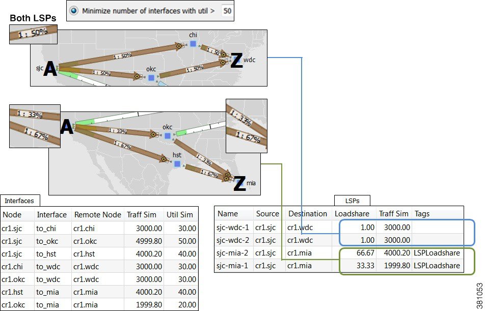
• Using the Acme_Network plan file (Figure 19-4), if you minimize the number of interfaces with utilization greater than 50%, only two of the Loadshare values change (Figure 19-6). Notice in the figure how Loadshare values are relative to the other Loadshare values for parallel LSPs, and not to all LSPs in the table. Also, only the affected LSPs are tagged.

Figure 19-4 Example Acme Network Before LSP Loadshare Optimization

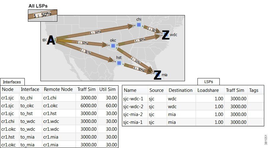
Figure 19-5 Example Acme Network After Minimizing Maximum Interface Utilization

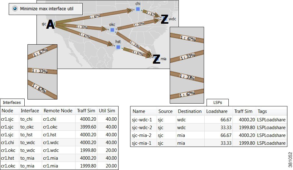
Figure 19-6 Example Acme Network After Minimizing Number of Interfaces with Utilization > 50%

Bin Example

In this example, a node uses a maximum of 32 bins, and the optimal traffic allocation is 45% of the traffic through LSP A and 55% of the traffic through LSP B. The node that sources these two LSPs, however, cannot do this exact split. The optimization divides the traffic into 32 bins, each with the same amount of traffic in them. Thus, each bin has 3.125% of the traffic (100% of the traffic divided by 32). The optimization also determines how the node should split the traffic. In this case, the split is to give 43.75% (which is 14 bins of 3.125% each) to LSP A and 56.25% (which is 18 bins of 3.125% each) to LSP B. Thus, it optimizes and distributes 32 (14+18) bins of traffic. This is as close as possible to the optimal 45%/55% split using 32 bins.

Workflow

The LSP Setup BW Optimization tool lets you add or remove LSPs based on set bandwidth requirements that you specify. You can select the LSPs that you want the optimizer to consider. The optimizer then separates these LSPs into different groups. The optimizer defines an LSP group based on the fact that the LSPs within the group share common source and destination nodes. You can also specify additional custom groupings to get a finer granularity on the setup bandwidth.

The optimizer lets you create LSPs by specifying:

• The number of LSPs to create for each LSP group.
• The maximum setup bandwidth per LSP. In this case, the minimum number of LSPs is created for each group in order to meet this requirement.

Additionally, the optimizer lets you remove LSPs by specifying:

• The number of LSPs to remove for each group.
• The minimum setup bandwidth per LSP. In this case, the minimum number of LSPs is removed from each group in order to meet this requirement.

You can then perform different operations on each group to test different design scenarios.

Note The sum of the setup bandwidth of the LSPs per group is not modified by adding or removing LSPs. The setup bandwidth is evenly redistributed among the LSPs within each LSP group.

Step 1 Choose Tools > RSVP LSP Optimization > LSP Setup BW Opt.

Step 2 Choose the LSPs you want the optimizer to consider. The default is to operate on all LSPs. If you want to consider just certain LSPs, choose a subset of the LSPs or choose tags to specify certain LSPs.

Step 3 Choose the manner in which LSPs are separated into LSP groups:

• Source/Destination Nodes—LSPs with a common source and destination belong in the same group.
• Source/Destination Nodes and existing SetupBWOpt::Group Entries—LSPs with a common source and destination and common SetupBWOpt::Group entries belong in the same group. This option is useful when you want to group LSPs based on different service classes.

Step 4 For each LSP group, provide your setup bandwidth requirements:

• Create x LSPs—Enter a positive integer. The optimizer creates a certain number of LSPs per group; for example, 1.
• Create the minimum number of LSPs so that Setup BW <= x Mbps—Specify the minimum number of LSPs to meet your setup bandwidth rule. For example, the bandwidth rule could be 10000 Mbps.
• Remove x LSPs—Enter a positive integer. The optimizer removes a certain number of LSPs per group; for example, 1.
• Remove the minimum number of LSPs so that Setup BW <= x Mbps—Specify the removal of the minimum number of LSPs to meet your setup bandwidth rule; for example, 10000 Mbps.

Step 5 (Optional) Override the defaults for how LSPs are tagged (SetupBWOpt) or for how new optimized plan files are saved.

Step 6 Click OK.

Summary Report

After running the LSP setup bandwidth optimization, the report summarizes the total number of:

• LSPs you selected.
• LSP groups identified.
• LSPs created.
• LSPs removed.

LSP Groups Report

In the Reports window, click LSP Groups to view details on how the optimizer operated on LSPs:

• Group—Name of the LSP group as specified by SetupBWOpt::Group. If this group is not specified, the Group column is empty.
• LSP Source—Source node of the LSP group.
• LSP Destination—Destination node of the LSP group.
• Total Setup BW—Sum of the setup bandwidth values of the LSPs within the LSP group.
• LSP Number Before—Number of LSPs within the LSP group before running the optimization.
• LSP Number After—Number of LSPs within the LSP group after the optimization.
• LSP Setup BW Before—Average setup bandwidth within the LSP group before the optimization.
• LSP Setup BW After—Setup bandwidth within the LSP group after the optimization.