Cisco Crosswork Hierarchical Controller 7.0 Assurance and Performance Guide
Available Languages
Bias-Free Language
The documentation set for this product strives to use bias-free language. For the purposes of this documentation set, bias-free is defined as language that does not imply discrimination based on age, disability, gender, racial identity, ethnic identity, sexual orientation, socioeconomic status, and intersectionality. Exceptions may be present in the documentation due to language that is hardcoded in the user interfaces of the product software, language used based on RFP documentation, or language that is used by a referenced third-party product. Learn more about how Cisco is using Inclusive Language.
- US/Canada 800-553-2447
- Worldwide Support Phone Numbers
- All Tools
 Feedback
 Feedback
This document is a how-to-use guide for Cisco Crosswork Hierarchical Controller assurance.
The following table lists the assurance applications. The Legend column indicates if the application falls into one of the following categories:
● Common: Common to all layers and multi-layer
● IP: Relevant to IP links and services
● Optical: Relevant to fibers, optical links, OTN/ETH connections
Table 1. Assurance Applications
| Category |
Application name |
Legend |
Description |
| Assurance |
IP |
Traffic utilization and OAM PM of port, links, tunnels and VPNs, group links by topology context (all LAG members, between router A to B), prediction of packet traffic utilization. |
|
| Optical |
L0-L1 performance, show correlation between photonic to L1 layer. Show power level across a span of ROADMs and Amplifiers. |
||
| Common |
Visualize L1-L2-L3 service configuration and underlay paths, with UNIs performance and events history. |
||
| Optical |
Visualize RON links across ZR and OLS with performance in all layers. |
||
| IP |
Calculate, on demand, an IGP path between two routers, visualize path and show performance of IP links across the path. |
||
| Common |
Show which services and links in the upper layers were impacted by a lower layer link failure, especially in the case of a multi-layer where an optical link failure impacted IP links and services. |
Terms
| Term |
Definition |
| Adapter |
The software used by Crosswork Hierarchical Controller to connect to a device or to the manager, to collect information required by the network model and configure the device. |
| Agg link |
Agg is Link Aggregation Group (LAG) where multiple ETH links are grouped to create higher bandwidth and resilient link. |
| BGP |
Border Gateway Protocol |
| Circuit E-Line |
An Ethernet connection between two ETH client ports on Transponder or Muxponder over OTN signal. |
| CNC |
Crosswork Network Controller. |
| Device |
Optical network element, router, or microwave device. |
| Device Manager |
The application that manages the deployed adapters. |
| eMBB |
Enhanced Mobile Broadband. |
| ETH link |
ETH L2 link, spans from one ETH UNI port of an optical device to another, and rides on top of ODU. |
| ETH chain |
A link whose path is a chain of Ethernet links cross-subnet-connected (found using Crosswork Hierarchical Controller cross-mapping algorithm). Eth-chain is a replacement for R_PHYSICAL link in cases where one side of the link is in devices out of the scope discovered by Crosswork Hierarchical Controller. |
| Fiber segment |
Physical fiber line that spans from one passive fiber endpoint (manhole, splice etc.) to another and is used as a segment in a fiber link. |
| Fiber |
Chain of fiber segments that spans from one optical device to another. |
| IGP |
IGP is the link between two routers that carries IGP protocol messages. The link represents an IGP adjacency. |
| IP-MPLS |
IP multi-protocol label switching. |
| L3-VPN link |
The connection between two sites of a specific L3-VPN (can be a chain of LSP connections or IGP path). |
| L3 physical |
L3 physical is the physical link connecting two router ports. It may ride on top of an ETH link if the IP link is carried over the optical layer. |
| L3-VPN |
A virtual private network based on L3 routing for control and forwarding. |
| Logical link, IGP, LSP |
Logical link connects VLANs on two IP ports. |
| LSP |
Label Switched Path, used to carry MPLS traffic over a label-based path. LSP is the MPLS tunnel created between two routers over IGP links, with or without TE options. |
| NMC (OCH-NC, OTSiMC) |
NMC is the link between the xPonder facing ports on two ROADMs. This link is the underlay for OCH and it is an overlay on top of OMS links. This is relevant only for disaggregation cases where the ROADM and OT box are separated. |
| NMS |
Network Management System. |
| OC/OCG |
SONET/SDH links that span from one optical device to another and carry SONET/SDH lower bandwidth services, the links ride on top of OCH links and terminate in TDM client ports. |
| OCH |
OCH is a wavelength connection spanning between the client port one OT device (transponder, muxponder, regen) and another. 40 or 80 OCH links can be created on top of OMS links. The client port can be a TDM or ETH port. |
| ODU |
ODU links are sub-signals in OTU links. Each OTU links can carry multiple ODU links, and ODU links can be divided into finer granularity ODU links recursively. |
| OSPF |
Open Shortest Path First, an Interior Gateway Protocol between routers. |
| OTN-Line |
An OTN connection between two ODU client ports over OTN path. |
| OTS |
OTS is the physical link connecting one line amplifier or ROADM to another. An OTS can be created over a fiber link. |
| OTU |
OTU is the underlay link in OTN layer, used for ODU links. It can ride on top of an OCH. |
| Packet E-Line |
A point-to-point connection between two routers or transponders/muxponders over MPLS-TP or IP-MPLS. |
| PCC |
Path Computation Client. Delegated to controller. Router is responsible for initiating path setup and retains the control on path updates. |
| PCE |
Path Computation Element. Controller-initiated. |
| Radio Media |
The media layer as a carrier of radio channels. |
| Radio Channel |
Multiple radio channels can be on top of radio media, each channel represents a different ETH link with its own rate. |
| RD |
Route Distinguisher. |
| RSVP-TE |
Resource Reservation Protocol to control traffic engineered paths over MPLS network . |
| RT |
Route Target. |
| SCH |
A super-channel is an evolution of DWDM in which multiple, coherent optical carriers are combined to create a unified channel of a higher data rate, and which is brought into service in a single operational cycle. |
| SDN Controller |
Software that manages multiple routers or optical network elements. |
| SR Policy |
Segment Routing Policy. A segment routing path between two nodes, with mapping to the IGP links based on SIDs list. |
| STS |
Large and concatenated TDM circuit frame (such as STS-3c) into which ATM cells, IP packets, or Ethernet frames are placed. Rides on top of OC/OCG as optical carrier transmission rates. |
| uRLLC |
Ultra-Reliable Low Latency Communications. |
| VRF |
Virtual Routing Function, acts as a router in L3-VPN. |
| ZR Media |
The media layer as a carrier of ZR channels, on top of OCH link. |
| ZR Channel |
Multiple ZR channels can be on top of ZR media, each channel represents a different IP link with its own rate. |
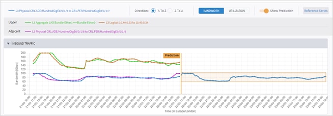
The Performance application provides statistical information on both packet-based traffic and optical (layer 0 and layer 1) performance:
● For layer 0 (OCH, NMC, OMS and OTS), provides Rx and Tx power data (minimum, average, and maximum).
● For layer 1 (ZR Media), provides Pre-FEC (Forwarding Error Correction), Post-FEC, Q Margin and Q Factor.
● For packet-based bandwidth traffic, the application provides statistical information on packet-based bandwidth/traffic usage of ports, links and LSPs over the selected time period. The information is calculated based on collected intervals/bins (15 minutes or 1 hour) of Rx and Tx octets and displayed in tables and in graphs.
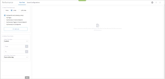
You can run a query by selecting resources and the time duration. This returns the Performance for the selected resources for a specified period and time window each day. A Performance test can be run explicitly on up to ten ports, links or LSPs by selecting the specific resources. The test can run on more ports and links by querying for ports, links or LSPs by tags or devices.
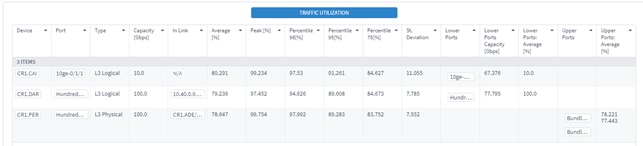
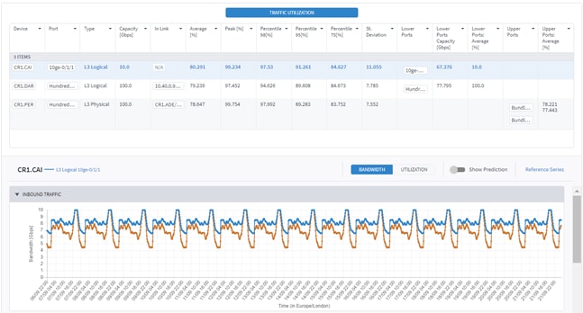
The displayed results include the resource capacity/speed and the statistical utilization info. Information on utilization is displayed for the selected resource and for the lower, upper, and adjacent resource, for example: logical ports on top of selected physical port, physical links lower to aggregation (LAG) link.
Resources can be selected explicitly by their type. After selecting the type, the user can use the model selector to select a resource (port, link or LSP). Ports, links or LSPs can also be selected by their tags, and routers (devices) can be selected using the model selector or by tag.
Utilization data is collected on IP links, for both physical and logical links. When links are selected, the user can select to view utilization for specific links/underlay (lower) links. If for example, an underlay link is selected, the application returns the utilization for both the underlay link itself and all the links above it that have utilization data.
It is also possible to view utilization data for links with devices in a single endpoint or links with devices in two endpoints. These endpoints can be defined by specific devices or by tags. For example, this allows the user to select a router and get the utilization data for all the links that end in this router or select two routers and get the utilization data for all the links between the two routers.
Using tags, means that the user can view utilization data for all links between devices with, for example, tag A, and devices with, for example, tag B.
Similarly, it is possible to select specific LSP/underlay links, as well as LSPs by devices in one or two endpoints.
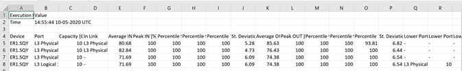
The capacity appears for ports and links, and the reserved bandwidth for LSPs. For all resources, the average utilization, peak utilization, various percentiles (98, 95 and 75), and standard deviation are shown. For ports, lower and upper port capacity and average utilization also appears, and for links the lower physical links, upper aggregate link, and upper logical links names are listed (if they exist).
You can select the following types of resources:
● Ports: Packet Ports, Optical Port, and ZR Ports
● Links: IP Links, Optical Links, and ZR Links
● LSPs: RSVP-TE tunnels and SR Policies.
The Traffic Utilization fields that appear vary according to the type of utilization being viewed.
Note: When selecting optical (layer 0 and 1) links, the Traffic Utilization tab appears with the information for the related L3 physical or logical layer.
For ports:
● Device
● Port
● Capacity [Gbps]
● In Link (if this exists)
● Average [%]
● Peak [%]
● Percentile 98[%]
● Percentile 95[%]
● Percentile 75[%]
● St. Deviation
● Lower Ports (only for logical port; aggregate or physical port name)
● Lower Ports Capacity [Gbps]
● Lower Ports Average [%]
● Upper Ports (only for physical port; the logical or aggregate port name, if exists)
● Upper Ports Average (%) (only for physical port)
For Ethernet and IP Links:
● Link
● Layer
● Capacity [Gbps]
● Average [%]
● Peak [%]
● Percentile 98[%]
● Percentile 95[%]
● Percentile 75[%]
● St. Deviation
● Lower Physical Links (link name of one layer lower, if exists)
● Upper Aggregate Link (link name, if exists)
● Upper Logical Links (link name, if exists)
For LSP Tunnels and LSP Policy Links:
● Link (full LSP name including site/device)
● Reserved BW [Mbps]
● Services (Traversing Over This LSP)
● Average Rate [Mbps]
● Peak Rate [Mbps]
● Percentile 98[Mbps]
● Percentile 95[Mbps]
● Percentile 75[Mbps]
● St. Deviation
Note: The export file includes extended information. The Average column appears in the UI, but in the export, there are two columns: Average IN and Average OUT. The UI shows the greater value of these two values.
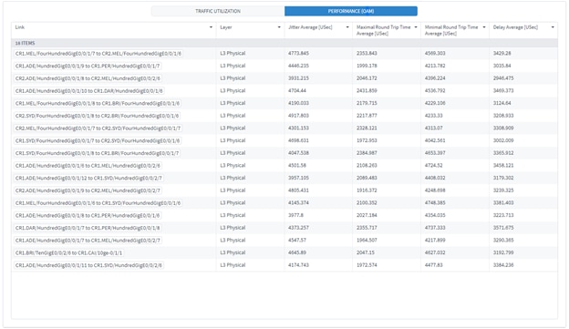
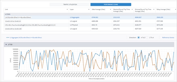
The following Performance fields appear for Ethernet and IP links:
● Link
● Layer
● Jitter Average (USec)
● Maximal Round Trip Time Average (Usec)
● Minimal Round Trip Time Average (Usec)
● Delay Average (Usec)
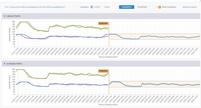
The Performance application has the option to predict the behavior of packet traffic utilization for the next 14 days based on the historical collection of performance monitoring counters. It is possible to view a prediction of packet traffic behavior assuming that you have at least 7 days of data available to base the prediction on.
The utilization graph can be opened per selected packet port or link (Ethernet or IP), and you can view the prediction as a linear line on the graph. The prediction is based on an algorithm that creates traffic patterns based on time of day, weekdays vs. weekends, and seasonal events in the local area where the system is deployed. The graph displays the linear utilization prediction line, as well as lower and upper bounds, indicating the prediction confidence interval. The prediction takes seasonal events into account.
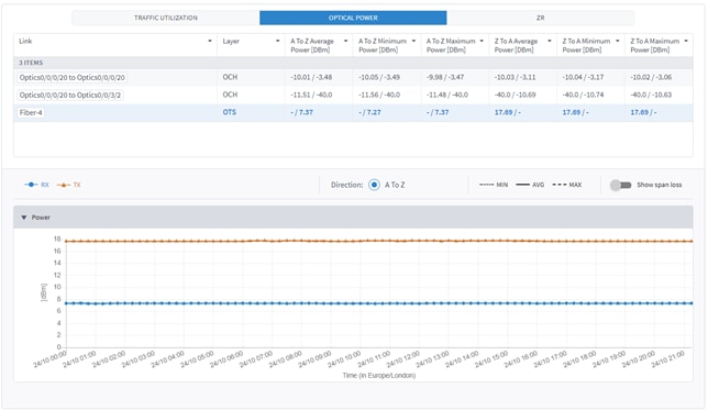
The Optical Power tab appears for layer 0 links (OTS, OMS, and OCH) and includes the following fields:
● Link
● Layer
● A to Z Average Power (DBm)
● A to Z Minimum Power (DBm)
● A to Z Maximum Power (DBm)
● Z to A Average Power (DBm)
● Z to A Minimum Power (DBm)
● Z to A Maximum Power (DBm)
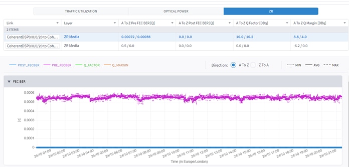
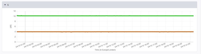
The ZR tab appears for layer 1 links (ZR Links) and includes the following fields:
● Link
● Layer
● A to Z Pre FEC BER (Q)
● A to Z Post FEC BER (Q)
● A to Z Q Factor (DBq)
● A to Z Q Margin (DBq)
Ports Traffic Utilization and Performance
You can view performance for Ethernet and IP ports:
● Specific ports
● Ports that are tagged with specific tags and tag values
● Ports on specific devices
● Ports by L3VPN Services
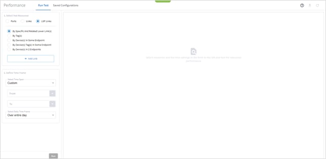
To configure performance for ports:
1. In the applications bar, select Performance.
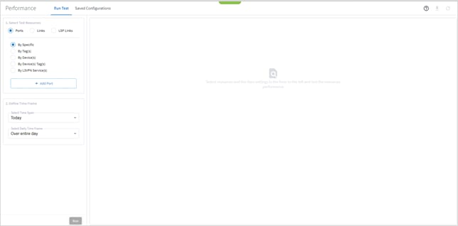
2. Ensure that Ports is selected.
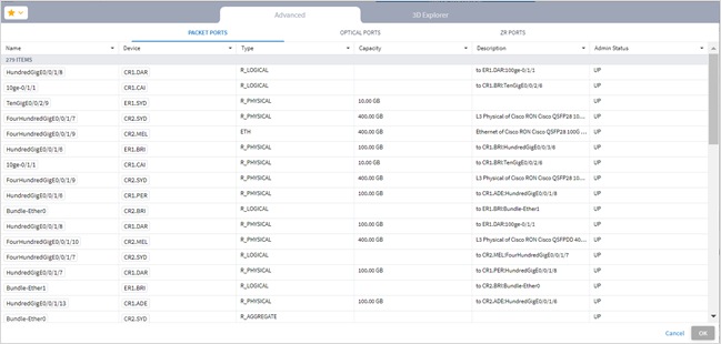
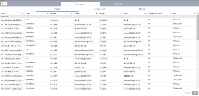
3. To check the performance for specific ports, select By Specific, and then click Add Port. In the Advanced tab, select from the Packet Ports, Optical Ports or ZR Ports tabs, or click on the 3D Explorer tab to select a port. Click OK. You can add up to 10 items.
Note: For more information on 3D Explorer, see the Cisco Crosswork Hierarchical Controller Network Visualization Guide.
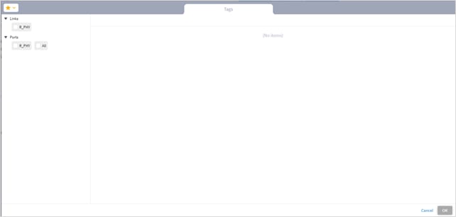
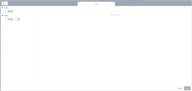
4. To check the performance for ports by tag, select By Tags(s), click Add Tag, and then select the tags and click OK.

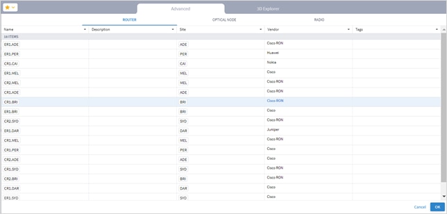
5. To check the performance for ports by device, select By Device(s), and then click Add Device. In the Advanced tab, select from the Router, Optical Node or Radio tabs, or click on the 3D Explorer tab to select a device. Click OK. You can add up to 10 items.

6. To check the performance for ports by device tag, select By Device(s) Tags(s), click Add Tag, and then select the tags and click OK.
7. To check the performance for ports by L3VPN services, select By L3VPN Services(s), and then click Add L3VPN Service. In the Advanced tab, select an L3VPN service, or click on the 3D Explorer tab to select a L3VPN service. Click OK. You can add up to 10 items.
8. Continue to View Utilization and Performance.
Links Traffic Utilization and Performance
You can view performance for:
● Specific and underlay links
● Links that are tagged with specific tags and tag values
● Links that include a device in a specific endpoint
● Links that include devices that are tagged with specific tags and tag values
● Links that include devices in two endpoints
To configure performance for links:
1. In the applications bar, select Performance.
2. Select Links.
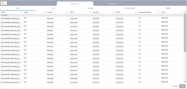
3. To check the performance for specific links, select By Specific And Underlay Lower Link(s), click Add Link, and then select a link. In the Advanced tab, select from the IP LINKS, OPTICAL LINKS or ZR LINKS tabs, or click on the 3D Explorer tab to select a link. Click OK. You can add up to 10 items.
Note: For more information on 3D Explorer, see the Cisco Crosswork Hierarchical Controller Network Visualization Guide.
4. To check the performance for links by tag, select By Tags(s), click Add Tag, and then select the tags and click OK.
5. To check the performance by devices in an endpoint, select By Device(s) In Some Endpoint, and then click Add Device. In the Advanced tab, select from the Router, Optical Node or Radio tabs, or click on the 3D Explorer tab to select a device. Click OK. You can add up to 10 items.

6. To check the performance for by device tag, select By Device(s) Tag(s) In Some Endpoint, click Add Tag, and then select the tags and click OK.
7. To check the performance for links with devices in two endpoints, select By Device(s) In 2 Endpoints and then select one of the following for Endpoint 1 and Endpoint 2.
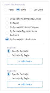
◦ Specific Device(s): Click Add Device and then select a device In the Advanced tab, select from the Router, Optical Node or Radio tabs, or click on the 3D Explorer tab to select a device. Click OK. You can add up to 10 items.
◦ Device(s) By Tag(s): Click Add Tag and then select the tags and click OK.
8. Continue to View Utilization and Performance.
LSP Links Traffic Utilization and Performance
You can view performance for:
● Specific LSP links
● LSP links that are tagged with specific tags and tag values
● LSP links that include a device in a specific endpoint
● LSP links that include devices that are tagged with specific tags and tag values
● LSP links that include devices in two endpoints
To configure performance for LSP links:
1. In the applications bar, select Performance.
2. Select LSP Links.
3. To check the performance for specific LSP links, select By Specific And Related Lower Link(s), click Add Link, and then select a link. In the Advanced tab, select from the LSP, IGP, IP Links, Optical Links or FIBER tabs, or click on the 3D Explorer tab to select a link. Click OK. You can add up to 10 items.
Note: For more information on 3D Explorer, see the Cisco Crosswork Hierarchical Controller Network Visualization Guide.
4. To check the performance for links by tag, select By Tags(s), click Add Tag, and then select the tags and click OK.
5. To check the performance by devices in an endpoint, select By Device(s) In Some Endpoint, and then click Add Device. In the Advanced tab, select from the ROUTER, OPTICAL NODE or RADIO tabs, or click on the 3D Explorer tab to select a device. Click OK. You can add up to 10 items.
6. To check the performance for by device tag, select By Device(s) Tag(s) In Some Endpoint, click Add Tag, and then select the tags and click OK.
7. To check the performance for links with devices in two endpoints, select By Device(s) In 2 Endpoints, and then select one of the following for Endpoint 1 and Endpoint 2.
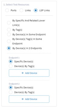
◦ Specific Device(s): Click Add Device and then select a device In the Advanced tab, select from the Router, Optical Node or Radio tabs, or click on the 3D Explorer tab to select a device. Click OK. You can add up to 10 items.
◦ Device(s) By Tag(s): Click Add Tag and then select the tags and click OK.
8. Continue to View Utilization and Performance.
View Traffic Utilization and Performance
After specifying the ports, links or LSP links, you must configure the time frame and window. You can then view the results in table and graph form.
To view performance:
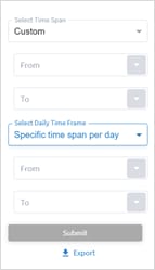
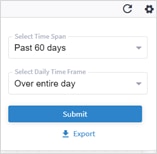
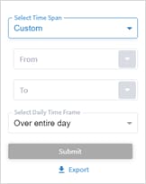
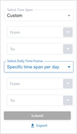
1. In the Select time area, specify the period to report on:
◦ Select Time Span: Select the required period, either Today, Past 24 hours, Past 7 days, Past 14 days, Past 30 days, Past 60 days, or Custom. If you select Custom, then click From and To and select a date and specify a time.
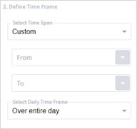
◦ In the Select Daily Time Frame area either select Over entire day or Specific time span per day. If you select Specific time span per day, then click From and Until to specify a time.
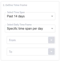
2. Click Run. If there are no relevant results, a Utilization information is not available for the selected resources message appears.
Note: When selecting optical (layer 0 and 1) links, the Traffic Utilization tab appears with the information for the related L3 physical, logical, or aggregate layers.
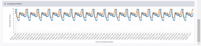
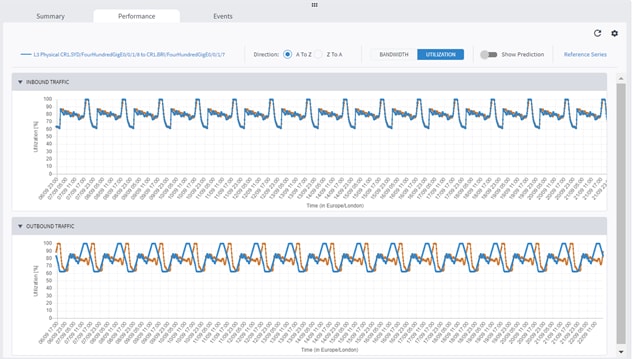
3. Select an item to see more details on the INBOUND TRAFFIC and OUTBOUND TRAFFIC.
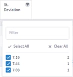
4. To filter the table, click ![]() and select the required options:
and select the required options:
◦ In numerical fields, the filter is numerical, and you can specify expressions including =, >, <, >=, <=, !=.
◦ In textual fields, the filter is character-based (regular expression).
5. To sort the table, click on a column heading.


6. In the TRAFFIC UTILIZATION tab, to change the y-axis scaling, click BANDWIDTH or UTILIZATION.
7. To view the prediction, select Show Prediction.
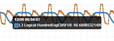
8. Hover over a data point on the graph to see the date, time, element name and utilization value.
9. To change the date range of the graph and zoom in or out, click on a graph and then using the mouse wheel, scroll up (to zoom in) or scroll down (to zoom out).
10. If you select to view the data over more than one day, for a specific time of day, for example, for the past 7 days between 13:00 and 15:00, the utilization graph appears with the values for the selected time window.
11. To view the reference series toggle, select Reference Series.
12. To remove a reference series, click on the series description.
![]()
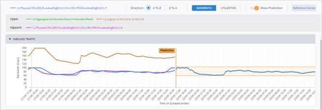
13. To change the direction, select A to Z or Z to A.
14. To view the OAM data (if relevant), click the PERFORMANCE (OAM) tab.
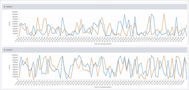
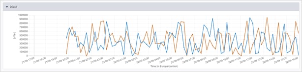
15. Select an item to see more details on JITTER, MIN RTT, MAX RTT, DELAY, and OUTBOUND TRAFFIC.
16. To view the optical data (if relevant), click the OPTICAL POWER tab. Select an item to see Power details.
17. To view the ZR media data (if relevant), click the ZR tab. Select an item to see FEC BER and Q details.
The tabular test results can be exported into a zip file with CSV files for offline analysis.
The export file includes extended information. The Average column appears in the UI, but in the export, there are two columns: Average IN and Average OUT. The UI shows the greater value of these two values.
To export the test results:
1. In the applications bar, select Performance.
2. Run the required test.
3. Click ![]() . The file is downloaded automatically.
. The file is downloaded automatically.
Manage Configurations
You can save the test configuration and either run the test when required or use it as a basis for a new test. You can also configure a test to run periodically.
To view a saved test result:
1. In the applications bar, select Performance.
2. Expand the required test.
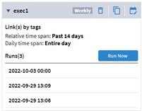
3. Select a run to view the results or click Run Now to execute the test.
To save a test configuration:
1. In the applications bar, select Performance.
2. Run the required test.
3. Click Save.
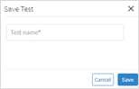
4. Enter a test name.
5. Click Save. The configuration is now available to run on the Saved Configurations tab.
To run a saved test configuration:
1. In the applications bar, select Performance.
2. Select the Saved Configurations tab.
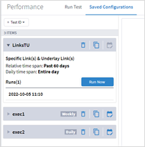
3. To run a test, expand the required test.
4. Click Run Now or if you want to edit the test, click ![]() , modify the test as required, and then click Run.
, modify the test as required, and then click Run.
To set a test to run periodically:
1. In the applications bar, select Performance.
2. Select the Saved Configurations tab.
3. For the required test, click ![]() .
.
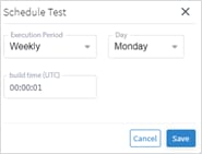
4. Select whether to execute the test Weekly (and on which day), or Daily.
5. Specify the build time (UTC).
6. Click Save.
To delete a test:
1. In the applications bar, select Performance.
2. Select the Saved Configurations tab.
3. Click ![]() . The test is deleted (there is no confirmation).
. The test is deleted (there is no confirmation).
Other Ways to See Performance Data
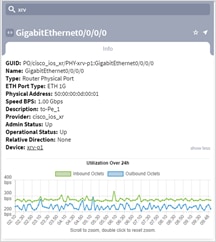
● In Explorer, for a physical or logical port of a router, the Utilization Over 24h graph also appears in the Info window (if the port was utilized over latest 24 hours). For links and LSP links no data is presented in the Explorer window.
● In the Service Assurance application, for point to point services. See View the Point to Point Services.
● In the Path Analysis application, for a path. See Analysis a Path.
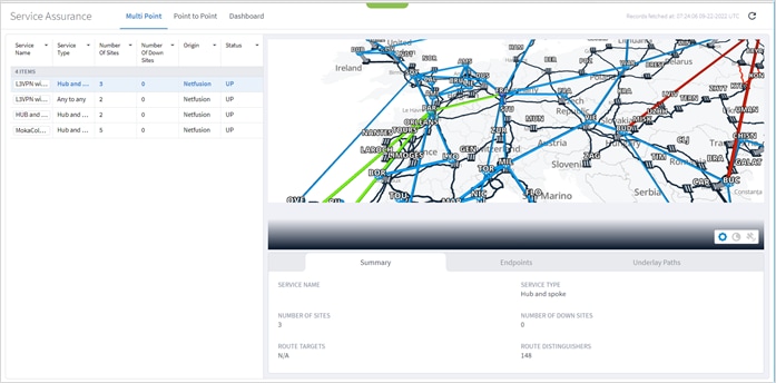
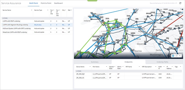
The Service Assurance application enables you to visualize the L1-L2-L3 service configuration and underlay paths, with UNIs performance and service-related events history.
For more information on services and service provision, see the Cisco Crosswork Hierarchical Controller Service Provisioning User Guide.
For more information on the 3D Explorer application, see the Cisco Crosswork Hierarchical Controller Network Visualization Guide.
Crosswork Hierarchical Controller discovers L3-VPN sites (endpoints), VRFs and underlay paths as LSPs across multiple domains (autonomous systems) and vendors and maps it to the optical network. Discovered VPNs are displayed in the Service Assurance application with their Route Distinguishers (RDs), Route Targets (RTs), type (hub & spoke or any to any/full mesh), sites, underlay LSPs and IGP path visualized on the map. The RD is used to keep all prefixes in the BGP table unique, and the RT is used to transfer routes between VRFs/VPNs.
You can view a list of these Multi Point services and view their endpoints and underlay paths. The Multi Point services can be of type:
● Any to any: A full mesh non-hierarchical service where any site can communicate with any site.
● Hub and spoke: A hierarchical service where hub sites can communicate with all other sites and spoke sites can only communicate with hub sites.
To view the Multi Point Services:
1. In the applications bar, select Service Assurance.
2. Select the Multi Point tab. The table on the left lists the multi point services and includes information on:
◦ Service Name: The name of the service as defined in the Services Manager.
◦ Service Type: The service type, Any to any or Hub and spoke.
◦ Number of Sites: The number of sites in the service.
◦ Number of Down Sites: The number of sites in the service that are DOWN.
◦ Origin: The origin of the service, either Netfusion (created by Crosswork Hierarchical Controller) or Network.
◦ Status: The service status, either UP or DOWN.
3. Select the required service. The Explorer map shows all sites and the underlay paths for the selected service.
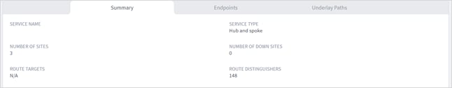
4. The Summary tab includes the following details:
◦ Service Name: The service name.
◦ Service Type: The service type, Any to any or Hub and spoke.
◦ Number of Sites: The number of sites in the service.
◦ Number of Down Sites: The number of sites in the service that are DOWN.
◦ Route Targets: The number of route targets.
◦ Route Distinguishers: The number of route distinguishers.
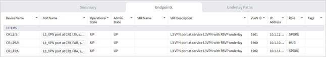
5. A list of the Endpoints appears below the map with the following details:
◦ Device Name: The device name.
◦ Port Name: The interface port name.
◦ Operational State: The operational status of the port (UP or DOWN).
◦ Admin State: The admin status of the port (UP or DOWN).
◦ VRF Name: The Virtual Routing and Forwarding (VRF) name.
◦ VRF Description: The VRF description.
◦ VLAN ID: The endpoint VLAN ID.
◦ IP Address: The endpoint IP address.
◦ Role: The role of the endpoint, SPOKE or HUB.
◦ Tags: The endpoint tags.
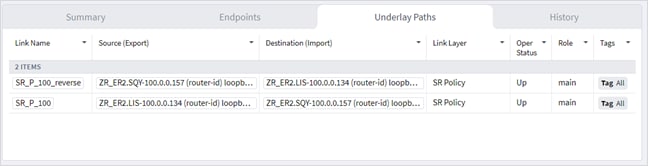
6. The Underlay Paths tab includes the following details:
◦ RT: The route target number.
◦ LSP Name: The LSP name (if RSVP-TE or LDP).
◦ Path Type: The type of the underlay path, SR Policies or RSVP-TE Tunnels.
◦ Source (Export): The source site name (geo site:device:port:vlan).
◦ Destination (Import): The destination site name (geo site:device:port:vlan).
◦ Underlay Hops: The number of hops in the underlay path.
◦ Link Layer: The link layer.
◦ Tags: The underlay tags.
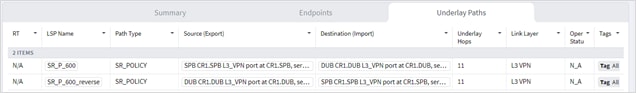
Note: Underlay paths are not discovered or calculated for sites located in different domains (inter-AS option C).
7. Select a path in the table to display it in the map.
View the Point to Point Services
You can view point to point services of type:
● Circuit E-Line: An Ethernet connection between two ETH client ports on Transponder or Muxponder over OTN signal.
● Packet E-Line: A point-to-point connection between two routers or transponders/muxponders over MPLS‑TP or IP‑MPLS.
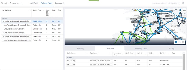
To view the point to point services:
1. In the applications bar, select Service Assurance.
2. Select the Point to Point tab. The table on the left lists the multi point services and includes information on:
◦ Service Name: The name of the service as defined in the Services Manager.
◦ Service Type: The service type, Packet e-line or Circuit e-line.
◦ Number of Down Sites: The number of sites in the service that are DOWN.
◦ Origin: The origin of the service.
◦ Status: The service status, either UP or DOWN.
3. Select the required service. The Explorer map shows the selected service.
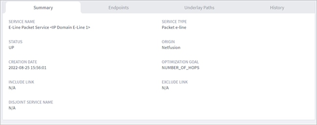
4. The Summary tab includes the following details:
◦ Service Name: The service name.
◦ Service Type: The service type, Packet e-line or Circuit e-line.
◦ Status: The service status, either UP or DOWN.
◦ Origin: The origin of the service.
◦ Creation Date: The date the service was created.
◦ Optimization Goal: The optimization goal as defined in the service.
◦ Include Link: The IP or optical links that were included in the service intent.
◦ Exclude Link: The IP or optical links that were excluded in the service intent.
◦ Disjoint Service Name: The disjoint service name. This means that the new Packet E-Line or Circuit E-Line must not traverse this exclusionary path (this would be equivalent to adding all the links that constitute the disjoint path to the exclude items from path list).
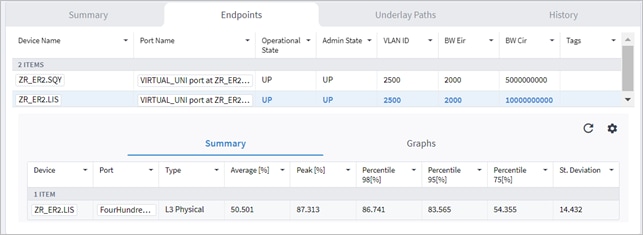
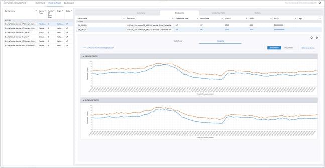
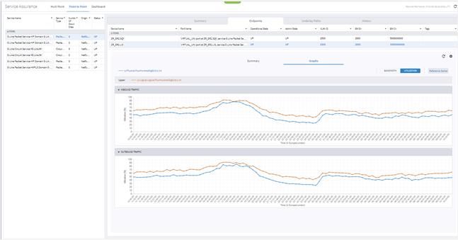
5. In the Endpoint tab, a list of the Endpoints appears below the map with the following details:
◦ Device Name: The device name.
◦ Port Name: The interface port name.
◦ Operational State: The operational status of the port (UP or DOWN).
◦ Admin State: The admin status of the port (UP or DOWN). If DOWN, this element constitutes a root cause failure in and of itself (and not simply an affected element).
◦ VLAN ID: The endpoint VLAN ID.
◦ BW Eir: The bandwidth Excess Information Rate (EIR).
◦ BW Cir: The bandwidth Committed Information Rate (CIR).
◦ Tags: The endpoint tags.
6. Select the required endpoint. The performance information appears for the selected service map with the following details:
◦ Device Name: The device name.
◦ Port: The port name.
◦ Type: The port name.
◦ Average [%]
◦ Peak [%]
◦ Percentile [98%]
◦ Percentile [95%]
◦ Percentile [75%]
● St Deviation
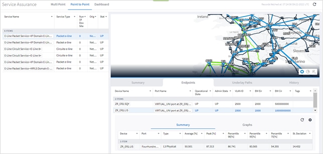
To view graphs of the performance, click the Graphs tab in the lower pane. For additional information on performance, see Performance.
7. Click ![]() and specify the period to report on:
and specify the period to report on:
◦ Select Time Span: Select the required period, either Today, Past 24 hours, Past 7 days, Past 14 days, Past 30 days, Past 60 days, or Custom. If you select Custom, then click From and To and select a date and specify a time.

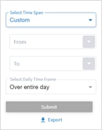
◦ In the Select Daily Time Frame area either select Over entire day or Specific time span per day. If you select Specific time span per day, then click From and Until to specify a time.
8. Click Export to download the performance statistics.
9. The Underlay Paths tab includes the following details:
◦ Link Name: The link name.
◦ Source (Export): The source site name (geo site:device:port:vlan).
◦ Destination (Import): The destination site name (geo site:device:port:vlan).
◦ Link Layer: The link layer. For Circuit e-line: ODU. For Packet e-line: MPLS TP, SR Policy, or LSP.
◦ Oper Status: The operational status.
◦ Role: Either the main path or the protection path.
◦ Tags: The underlay tags.
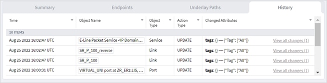
10. The History tab shows all changes in configuration or in operational status of the service and its underlay path links or tunnels and includes the following details:
◦ Time: The time of the event.
◦ Object Name: The object name.
◦ Object Type: The object type, port, service, or link.
◦ Action Type: The action type, UPDATE, INSERT or DELETE.
◦ Changed Attributes: The attributes changed.
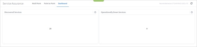
In the Dashboard you can see how many services were discovered and how many services are operationally down.
To view the Dashboard:
1. In the applications bar, select Service Assurance.
2. Select the Dashboard tab.
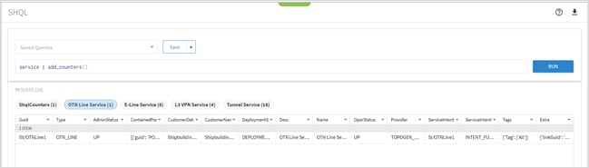
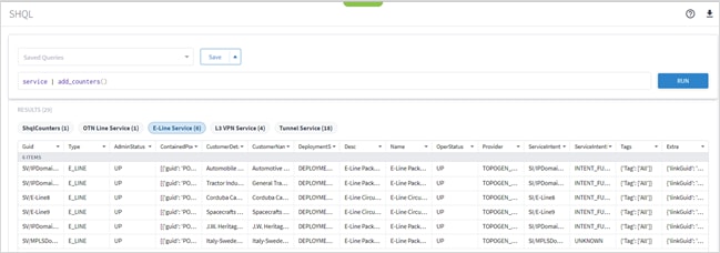
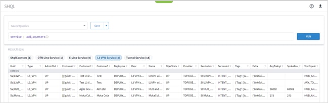
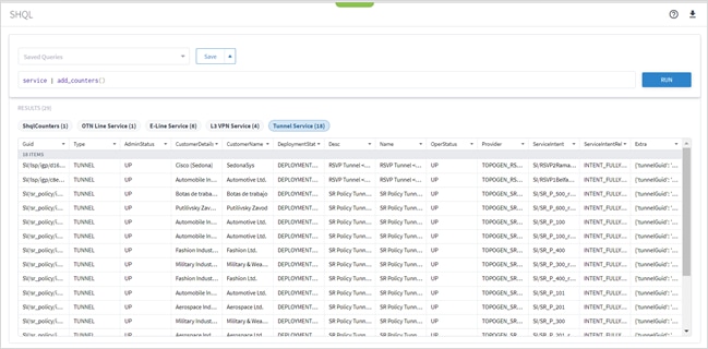
If you have access to SHQL, you can execute a query to view a list of the various services (by type).
To view the services using SHQL:
1. In the applications bar, select SHQL Query.
2. Enter service | add_counters() and click RUN. This shows you the total number of configured services.
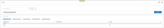
3. Click the required service tab to view a list of the services, for example, OTN Line Services, E-Line Services, L3 VPN Services, or Tunnel Services (RSVP Tunnel and SR Policy).
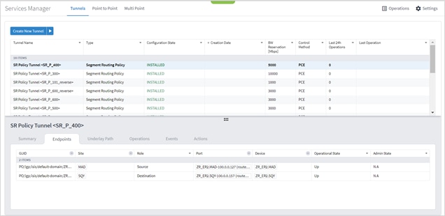
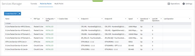
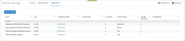
View the Services in Services Manager
Services Manager is an application that manages provisioning, modification, and deletion of services of all types. If you have access to Services Manager, you can view a list of the tunnels, point to point services, and multi point services.
Services Manager provides information on configuration of the services. It can help you view the status of user operations and to track mismatches between desired and actual configuration.
To view the services in Services Manager:
1. In the applications bar, select Services Manager.
2. Select the required tab.
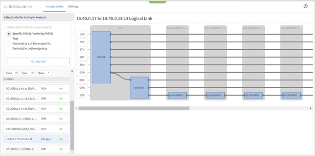
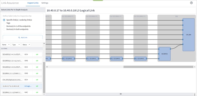
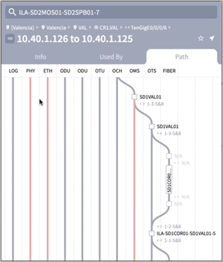
The Link Assurance application allows you to visualize any IP or Ethernet links across ZR and OLS with performance in all layers, that is, RON links. This all‑in-one app is used for analysis of router-to-router or OT-to-OT link across ZR/+ pluggables and optical line systems and enables you to view aggregated link status as propagated from all layers, and drill down to performance and events history per link.
To inspect links:
1. In the applications bar, select Link Assurance.
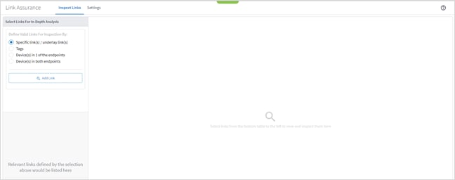
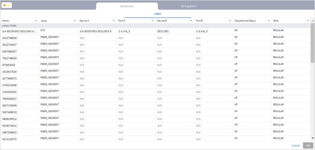
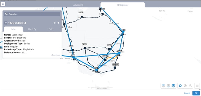
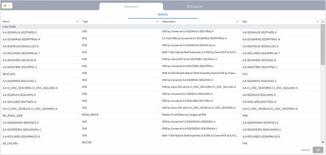
2. To inspect links for specific links/underlay links, select Specific link(s) / underlay link(s), click Add Link. In the Advanced tab, select a link in the LINKS tab, or click on the 3D Explorer tab to select a link (optical links are in black). Click OK. You can add up to 10 items.
Note: For more information on 3D Explorer, see the Cisco Crosswork Hierarchical Controller Network Visualization Guide.
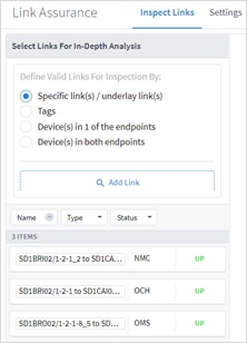
3. To inspect links by tag, select Tags, click Add Tag, and then select the tags and click OK.
4. To inspect links by endpoint, select Device(s) in 1 of the endpoints, and then click Add Endpoint. In the Advanced tab, select a device in the DEVICES tabs, or click on the 3D Explorer tab to select a device. Click OK. You can add up to 10 items.
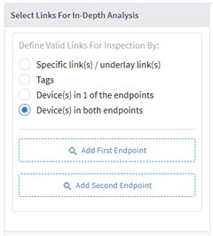
5. To check the performance for links with devices in two endpoints, select Device(s) in both endpoints and then click Add First Endpoint and select a device. Repeat for the second endpoint.
6. Continue to View Links and Performance.
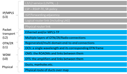
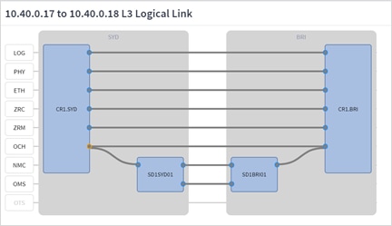
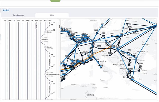
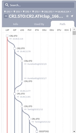
After specifying the links, you can select one of the links in the list on the left and view the hierarchy of the link layers on the right.
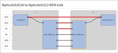
Legend:
● Blue Filled Rectangle: Node or router
● Lines: Links
● Circles: Ports
● Grey fill: Up
● Red fill: Down
● Blue Frame: Not selected
● Orange Frame: Selected
To view links:
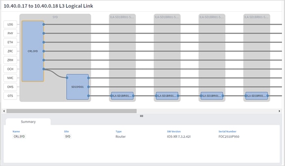
1. Select one of the link layers. You can scroll left and right to see the full path.
2. Click on a layer name to exclude the layer from the view. For example, click on OTS.
![]()
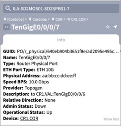
3. Click the blue square representing a router or optical node to view the details for the router or optical node. The router or optical node is framed in orange. The Summary tab includes the following details:
◦ Name: The name of the router or optical mode.
◦ Site: The site name.
◦ Type: Router or Optical Node.
◦ SW Version: The software version on the router.
◦ Serial Number: The router or optical node serial number.
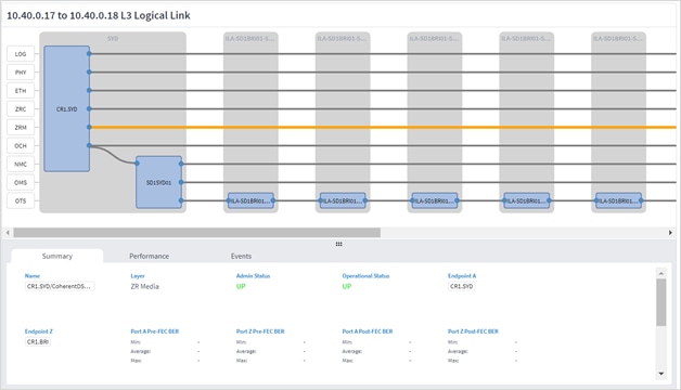
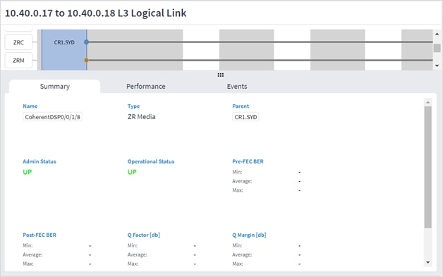
4. Click the line representing the link to view the link details. The selected link is orange. The Summary tab includes the following details:
◦ Name: The name of the link.
◦ Layer: The layer type: L3 Logical, L3 Physical, Ethernet, ZR Channel, ZR Media, OCH, NMC, OMS or OTS.
◦ Admin Status: The admin status: UP or DOWN.
◦ Operational Status: The operational status: UP or DOWN.
◦ Endpoint A: The starting endpoint.
◦ Endpoint Z: The terminating endpoint.
◦ For Ethernet links, the rate for Port A Rate [Gbps] and Port A Rate [Gbps].
◦ For ZRM links, the min, average and max values for Port A Pre-FEC BER, Port Z Pre-FEC BER, Port A Pre-FEC BER and Port Z Pre-FEC BER.
◦ For OCH, NMC, OMS, and OTS links, the min, average and max values for Port A Tx Power [dbm], Port Z Tx Power [dbm], Port A Rx Power [dbm] and Port Z Rx Power [dbm].
5. For Ethernet and IP links or ports the Performance tab includes INBOUND TRAFFIC and OUTBOUND TRAFFIC graphs for BANDWIDTH and UTILIZATION.
For additional information on performance, see Performance.
6. Click ![]() and specify the period to report on:
and specify the period to report on:
◦ Select Time Span: Select the required period, either Today, Past 24 hours, Past 7 days, Past 14 days, Past 30 days, Past 60 days, or Custom. If you select Custom, then click From and To and select a date and specify a time.
◦ In the Select Daily Time Frame area either select Over entire day or Specific time span per day. If you select Specific time span per day, then click From and Until to specify a time.
7. Click Export to download the performance statistics.
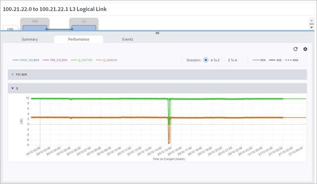
8. For layer 1 (ZR Media), the Performance tab includes Post_FECBER, Pre_FECBER, Q_Factor and Q_Margin.
For additional information on performance, see Performance.
9. For layer 0 (OCH, NMC, OMS and OTS), the Performance tab includes Rx and Tx power data.
For additional information on performance, see Performance.
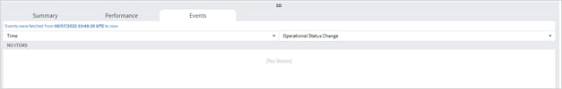
10. The Events tab includes a list of the operational status changes.
11. Click the port to view the related summary, performance, and events.
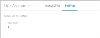
● The Days Back setting applies to the statistics data for the Summary and Performance tabs. Use this configuration to apply the Days Back to Performance tabs of all ports and links that can be selected, without having to repeat the settings for every port/link.
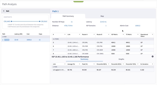
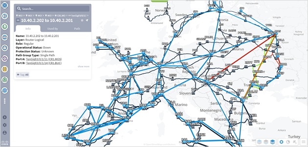
This application analyses the potential IGP paths between two endpoints. Each path is analyzed and broken down into links, and the cost of each path is calculated. The path-selection decision is based on the minimum cost, where the cost is the total of the IGP metric values for the links in the path. All paths with a similar cost are returned.
Dynamic paths such as LDP and SR-ISIS, over IGP links, are supported (where no path preferences are provided).
Table 2. Path Analysis Terms
| Term |
Definition |
| Cost |
The accumulated IGP metric for the path, that is, sum of the IGP metrics of the various links in the path. |
| Hops |
The number of links in the path. |
| IGP Metric |
The hop IGP metric. |
| Latency |
The total latency of the links in the path. |
| TE Metric |
The hop TE tunnel metric. |
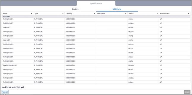
To analyze a path, select two endpoints. Endpoints can be a router or UNI port connected to a VPN service. The application returns all the alternate paths with the same minimum cost, where cost is defined as the aggregation of the IGP Metrics for the links in the path. Related performance data can be viewed for the logical IP links in the path.
To analyze a path:
1. In the applications bar, select Path Analysis.
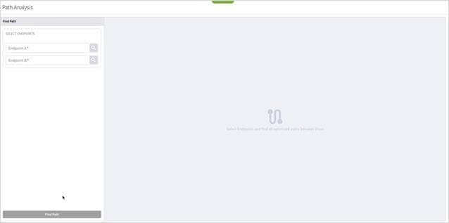
2. Click ![]() to add a router as endpoint A.
to add a router as endpoint A.
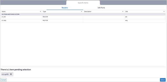
3. (Optional) Select the UNI Ports tab.
4. Select an endpoint and click OK.
5. Repeat to select endpoint B. A list of the paths with the same cost appears.
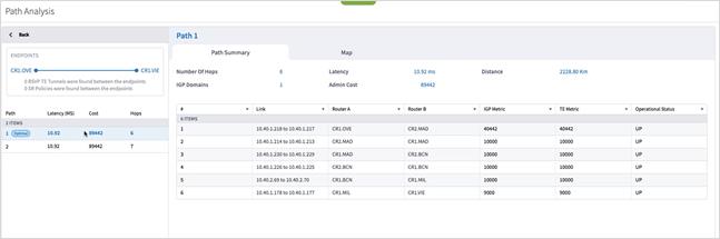
6. Click on a path to see the number of hops, latency, distance, number of IGP domains and admin cost for the path. The table details each of the links with their endpoint routers, IGP metric and TE metric.
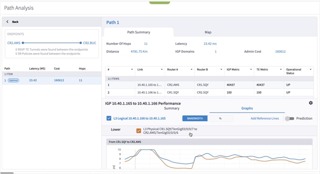
7. Click on a link in the path to see the related performance information. The information appears in the Summary tab in the lower pane.
8. To view graphs of the performance, click the Graphs tab in the lower pane. For additional information on performance, see Performance.
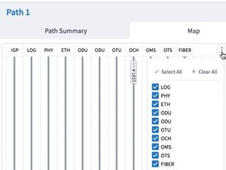
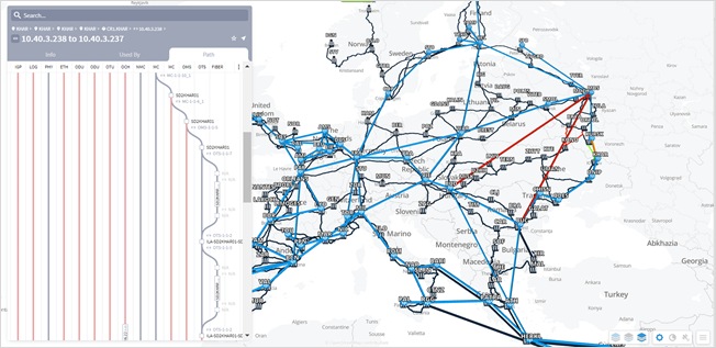
9. Click the Map tab to view the path in the 3D Explorer map.
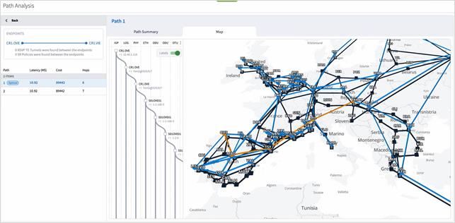
10. You can expand and scroll in the Metro view to see more of the path details.
11. You can also filter the path as required.
The Root Cause Analysis application finds the failed lower layer links that are the root cause of a link or a service failure. To establish root cause failures, Crosswork Hierarchical Controller considers both the operational status (up/down) of the links and the admin status (up/down) of the router ports.
When the operational status of a link is down, this is considered a failure. Crosswork Hierarchical Controller then checks all the lower layer links that have failed, until the element at the lowest level is identified. This is the root cause element. All elements above this root cause element are considered affected elements. A link with operational status down but with no links above it is still considered as a root cause.
If an element has an admin status of down, it is classified as a root cause element (and not as an affected element).
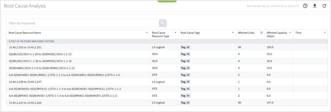
You can view a list of the root causes and can view the:
● Root cause resource type: L3 Logical, OCH, OTS, LSP, or OMS.
● Root cause tags
● Number of affected links
● Affected capacity (Gbps)
● Time
● A list of the link layers and elements affected
You can also hover over the affected element to view the element in the map (and then view the element in Explorer) or click on the element name to drilldown directly to the element in Explorer.
Table 3. Elements
| Links |
Description |
| LSP |
The MPLS tunnel created between two routers over IGP links, with or without TE options. |
| IGP |
The link between two routers that carries IGP protocol messages. The link represents an IGP adjacency. |
| L3 Logical (R_LOGICAL) |
A link that connects VLANs on two IP ports. |
| L3 Physical (R_PHYSICAL) |
The physical link connecting two router ports. It may ride on top of an ETH link if the IP link is carried over the optical layer. |
| Ethernet (ETH) |
An ETH L2 link, spans from one ETH UNI port of an optical device to another, and rides on top of ODU. |
| ODU |
ODU links are sub signals in OTU links. Each OTU link can carry multiple ODU links, and ODU links can be divided into finer granularity ODU links recursively. |
| OTU |
The underlay link in the OTN layer, used for ODU links. It can ride on top of an OCH. |
| OCH |
A wavelength connection spanning the client port of one OEO device (transponder, muxponder, regen) and another. 40 or 80 OCH links can be created on top of OMS links. The client port can be TDM or ETH port. |
| OMS |
The link connecting one ROADM to another. One OMS can be created over a chain of OTS links. |
| OTS |
The physical link connecting between one line amplifier or ROADM and another. One OTS can be created over a fiber link. |
For more information on Explorer and the various links, see the Cisco Crosswork Hierarchical Controller Network Visualization Guide.
To view root cause failures:
1. In the applications bar, select RCA. A list of the root causes appears with the following information:
◦ Root Cause Resource Name: The root cause link name. In this example, the OTS link.
◦ Root Cause Resource Type: The root cause link type.
◦ Root Cause Tags: The root cause tags.
◦ Affected Links: The total number of elements affected by this root cause.
◦ Affected Capacity (Gbps): The total bandwidth lost in Gbps (the total of all links).
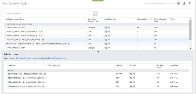
2. Select the required root cause. Detailed information for the root cause appears.
3. Hover over the root cause resource name and click ![]() to view the root cause in the map.
to view the root cause in the map.
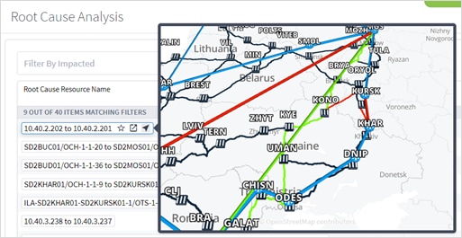
4. Click ![]() Open in Explorer to open the root cause in Explorer.
Open in Explorer to open the root cause in Explorer.
5. You can navigate up and down the link layers by clicking on the Used By tab.
6. In the Used By tab, click on the link name.
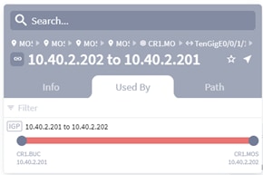
7. Repeat this to navigate to the next layer.
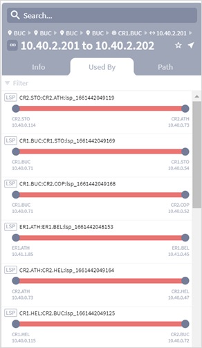
8. Continue until you get to the uppermost layer. The Explorer map is updated as you navigate.
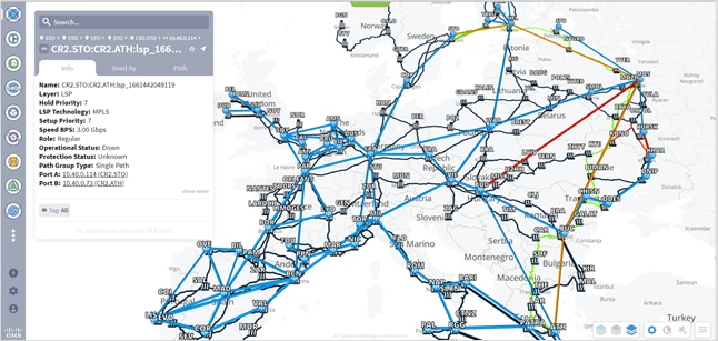
9. Select the Path tab to view the layers.
10. In this example, there are two root cause failures. The Ethernet root cause failure affects the PHY layer above it, but the OMS root cause failure does not affect any of the links above it and so there are 0 affected elements.
11. In this example, the root cause failure affects two links, the MC and OMS links.
12. In this example, there is an Admin Status: Down. This means that this element constitutes a root cause failure in and of itself (and not simply an affected element).
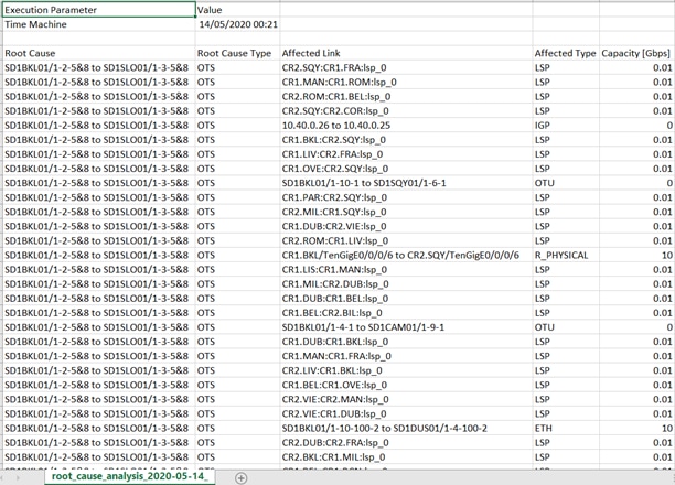
You can download a comma separated file with the root cause information.
To download root causes:
1. In the applications bar, select RCA.
2. Click ![]() . A root_cause_analysis_<date>.csv file is downloaded.
. A root_cause_analysis_<date>.csv file is downloaded.
3. Open the downloaded file to view a list of the root causes appears with the following information:
◦ Root Cause: The root cause link name. In this example, the OTS link.
◦ Root Cause Type: The root cause link type.
◦ Affected Link: The link affected by this root cause.
◦ Affected Type: The type of the link affected by this root cause.
◦ Capacity [Gbps]: The bandwidth lost in Gb for the affected link.
![]()