Optimize LSPs

This section contains the following topics:

Optimize Disjoint LSP Paths

LSPs and LSP paths are disjoint if they do not route over common objects, such as interfaces, or nodes. The LSP disjoint path optimization tool (Actions > Tools > LSP optimization > LSP disjoint path optimization) creates disjoint LSP paths for RSVP LSPs and SR LSPs, and optimizes these paths based on user-specified constraints.


Note


The LSP disjoint path optimization tool supports both Inter-Area and Inter-AS functionalities.


One common use case for this optimization is that disjoint LSPs can ensure that the services are highly resilient when network failures occur. For example, this tool lets you route LSPs to have disjoint primary and secondary paths that are optimized to use the lowest delay metric possible.

If it is not possible to achieve the optimization as defined by the routing selection, path requirements, and constraints, the tool provides the best disjoint paths and optimization possible.

Upon completion, by default, Cisco Crosswork Planning tags the LSPs with DSJOpt and writes a report containing the results of the optimization.


Note


While the optimizer applies to both RSVP LSPs and SR LSPs, only one of these types of LSPs can be optimized at a time.

Specify Optimization Inputs

Disjoint Routing Selection

In Cisco Crosswork Planning, only existing LSP paths are rerouted. New LSP paths are not created.

  • Explicit hops are modified or created for RSVP LSPs.

  • Segment list hops are modified or created for SR LSPs. The final hop is either a node hop or interface whose remote node is the destination of the LSP.

Segment lists are created only for LSP paths, and only LSP path segment lists are updated. If a segment list is associated with an LSP (rather than an LSP path), that LSP segment list is removed.

Figure 1. Disjoint Routing Selection Options

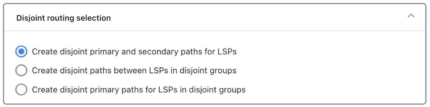
Routing options include:

  • Create disjoint primary and secondary paths for LSPs—For all LSPs, whether they are in a disjoint group or not, routes all LSP paths so that they are disjoint from all other paths belonging to that LSP. This disjointness extends beyond primary and secondary paths to include all other path options (for example, tertiary).

  • Create disjoint paths between LSPs in disjoint groups—For all LSPs that are in disjoint groups, routes all LSP paths so that they are disjoint from all other paths belonging to LSPs in that disjoint group. This disjointness extends beyond primary and secondary paths to include all other path options (for example, tertiary).

    Example: All LSPs in disjoint group East are rerouted to be disjoint from each other. All LSPs in disjoint group Southeast are rerouted to be disjoint from each other. However, LSP paths in the East group are not rerouted to be disjoint from those in the Southeast group.

  • Create disjoint primary paths for LSPs in disjoint groups—For all LSPs that are in disjoint groups, reroutes only their primary paths so that they are disjoint from each other.

Disjoint Path Requirements

The disjoint path requirements identify the priority for creating disjointness across a path. Disjointness priorities 1, 2, 3, and Ignore are available for circuits, SRLGs, nodes, and sites. The tool tries to create disjointness for all objects that have a priority set other than Ignore. If full disjointness cannot be achieved, the tool prioritizes disjointness based on these values.

Figure 2. Disjoint Path Requirements

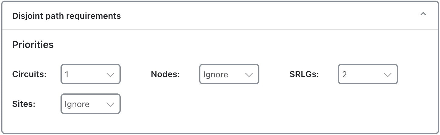
For example, in Disjoint Path Requirements, Circuits have a priority of 1, SRLGs have a priority of 2, and the other objects are ignored. If the tool cannot achieve full disjointness across both circuits and SRLGs, it prioritizes the disjointness of circuits over SRLGs.

Example

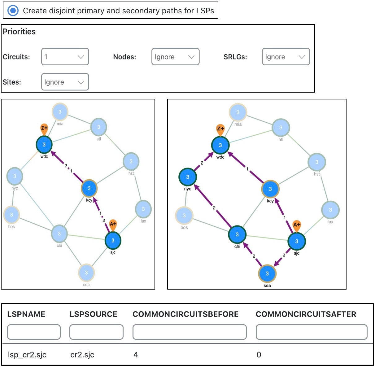
This example shows how disjoint routes can be created for primary and secondary RSVP LSP paths, and how those routes differ, depending on the path requirements set. The LSP has a primary and secondary LSP paths that use the same route from cr2.sjc to cr2.wdc. The LSP is not a member of a disjoint group.

The Primary and Secondary Paths Based on Disjoint Circuit Requirements shows the different route from cr2.sjc to cr2.wdc. Because the disjoint path requirement is only circuits, the primary and secondary paths route across different circuits, as indicated in the resulting report.

Figure 3. Primary and Secondary Paths Based on Disjoint Circuit Requirements

Constraints

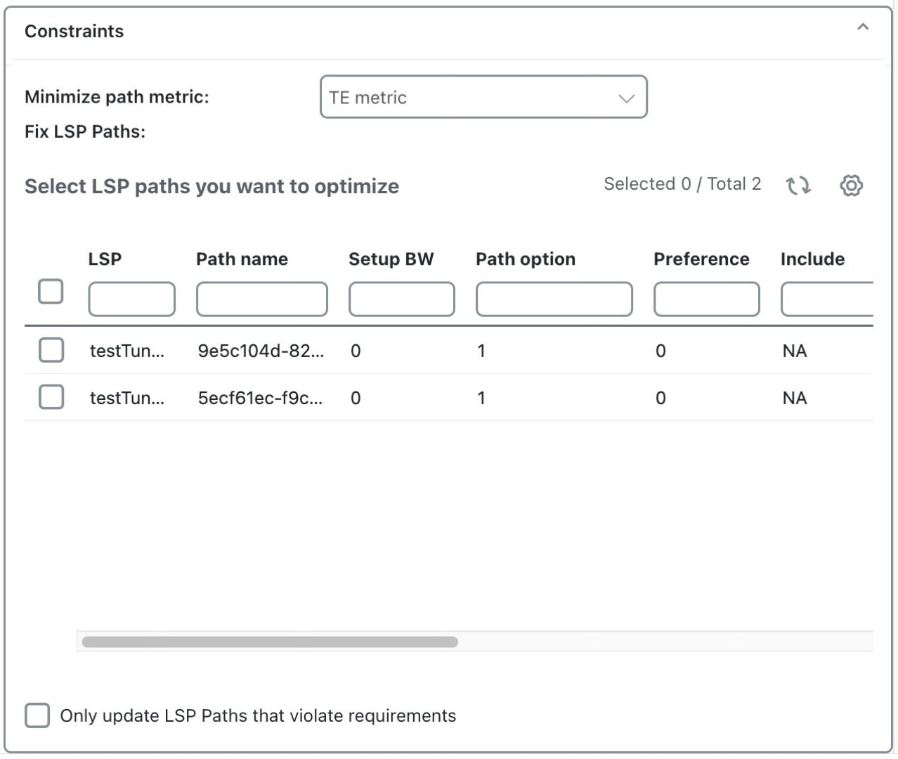
Following options are available in the Constraints section:

  • Minimize path metric—Paths are optimized to minimize the sum of the metrics along the path with respect to delay, TE, or IGP metrics. All of these properties are configurable from an interface Properties window, and delays can also be set in a circuit Properties window.

  • Fix LSP Paths—Selected or tagged LSP paths are not rerouted. This constraint is useful when you have previously optimized specific LSPs within the network and want to maintain their routes.

  • Only update LSP Paths that violate requirements—Paths are modified only if they violate the requirements specified in the area of the Disjoint Path Requirements window.

Example

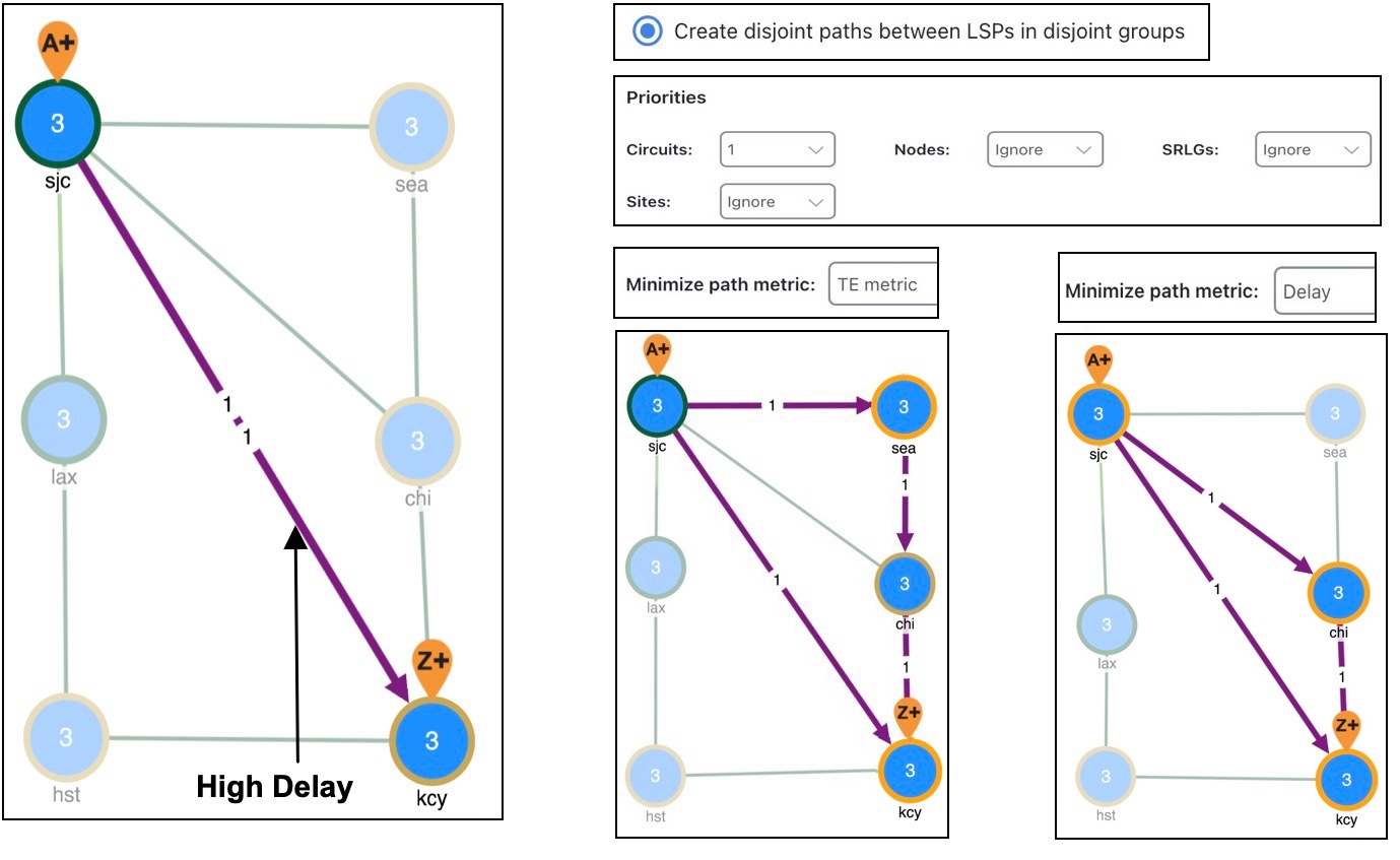
This example shows how disjoint routes can be optimized for two SR LSPs using the same source (sjc) and destination (kcy).

  • Both LSPs belong to the same disjoint group, and both LSPs have an LSP path.

  • The circuit between sjc and kcy has significantly higher delay than the other circuits.

  • The only disjoint path requirement selected is circuits.

  • Example Routing of SR LSPs shows the following:

    • Before using the LSP Disjoint Path Optimization tool, both LSP paths use the same route. There are no segment list hops.

    • By selecting the option to create disjoint paths between LSPs in the same disjoint group and using the TE metric for the shortest path calculation, two disjoint LSP path routes are created. Both have a segment list node hop (as indicated by the orange circle around the node) on the destination node. One has an additional segment list node hop on sea to force a different route.

    • By selecting the same disjoint option and using the Delay metric for the shortest path calculation, one LSP is moved away from the high-delay sjc-kcy circuit because traversing that circuit is not the shortest latency path.

Figure 4. Example Routing of SR LSPs

Create Disjoint Groups

Before you begin
  • The network model must already contain the primary LSP paths. If using the option to create disjoint primary and secondary paths, it must also at least contain secondary LSP paths, though it can contain other path options, such as tertiary.

  • If creating disjoint paths between LSPs in the same disjoint group, the LSPs must first be added to the disjoint groups.

Procedure

Step 1

Open the plan file (see Open Plan Files). The plan file opens in the Network Design page.

Step 2

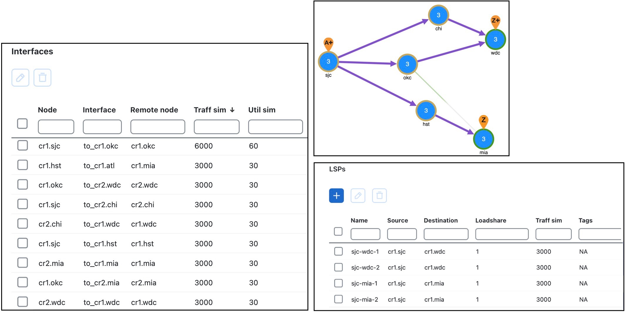
In the Network Summary panel on the right side, choose one or more LSPs from the LSPs table.

Step 3

Click Edit icon.

Step 4

Click the Advanced tab.

Step 5

Expand the Explicit route selection panel and enter the Disjoint group name.

Step 6

Assign priorities to LSPs within these groups, if needed. Higher priority LSPs are assigned shorter routes based on the selected metric. The higher the number, the lower the priority.

Example: There are two LSPs in the same disjoint group, each with a different disjoint priority. Run the LSP disjoint path optimization tool to create disjoint paths for LSPs in the same disjoint group using TE metrics as a constraint. The LSP with a disjoint priority of 1 routes using the lowest TE metric, and the LSP with a disjoint priority of 2 routes using the second lowest TE metric.

Step 7

Click Save.


Run the LSP Disjoint Path Optimization Tool

To run the LSP disjoint path optimization tool, do the following:
Procedure

Step 1

Open the plan file (see Open Plan Files). The plan file opens in the Network Design page.

Step 2

From the toolbar, choose any of the following options:

  • Actions > Tools > LSP optimization > LSP disjoint path optimization

    OR

  • Preset workflows > Perform optimization, select LSP Optimization as the optimization type, choose LSP disjoint path optimization from the drop-down list, and click Launch.

Step 3

Select the LSPs for which you want to optimize the disjoint paths.

Step 4

Click Next.

Step 5

In the Disjoint routing selection section, select how to route the disjoint paths. For details, see Disjoint Routing Selection.

Step 6

In the Disjoint path requirements section, select the disjoint path requirements and priorities. For details, see Disjoint Path Requirements.

Step 7

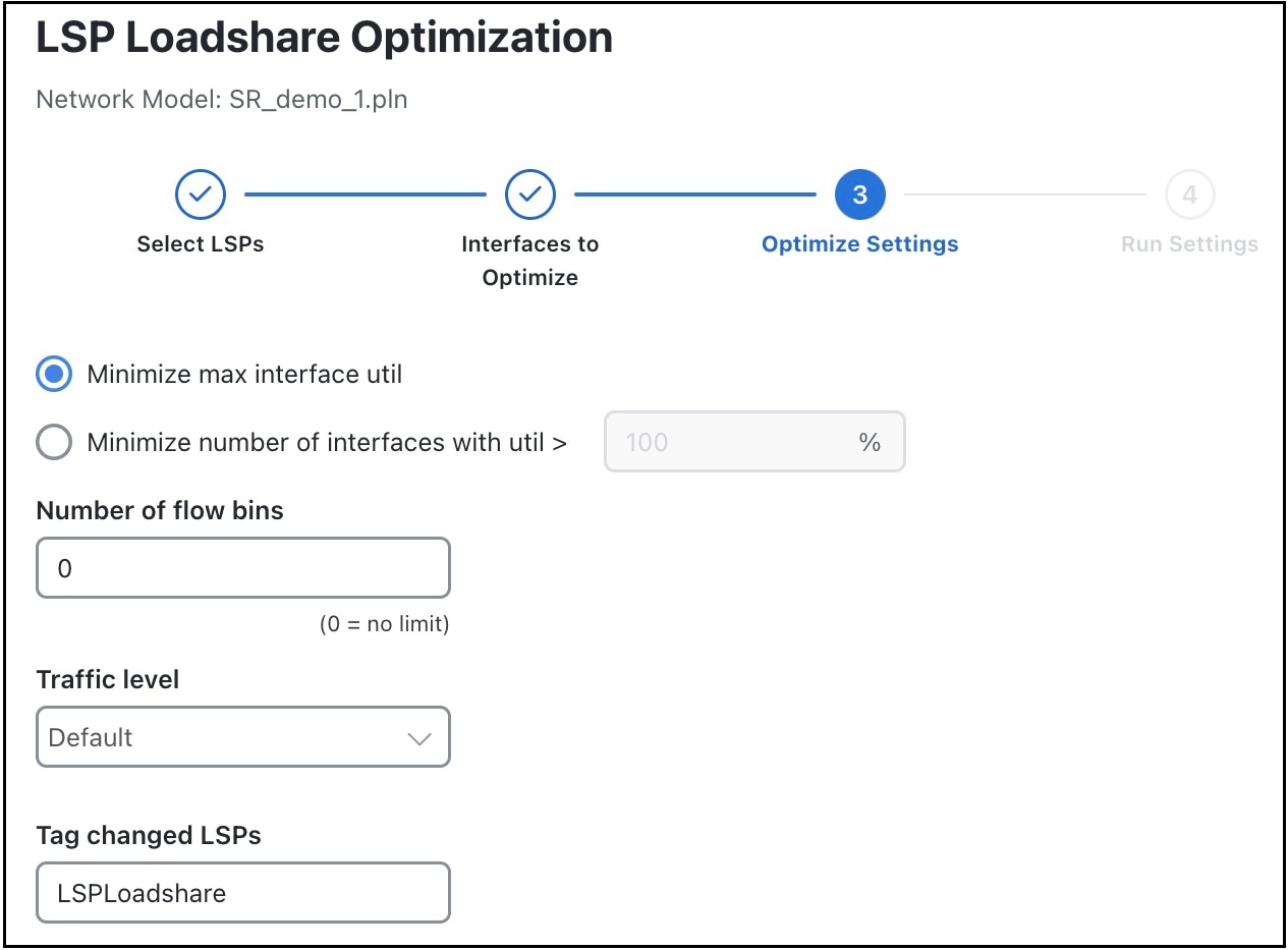
In the Constraints section, select the constraints. For details, see Constraints.

Step 8

Click Next.

Step 9

(Optional) In the Tag updated LSP Paths with field on the Run Settings page, override the defaults for how LSP paths are tagged (DSJopt).

Step 10

On the Run Settings page, choose whether to execute the task now or schedule it for a later time. Choose from the following Execute options:

  • Now—Choose this option to execute the job immediately. The tool is run and changes are applied on the network model immediately. Also, a summary report is displayed. You can access the report any time later using Actions > Reports > Generated reports option.

  • As a scheduled job—Choose this option to execute the task as an asynchronous job. If you choose this option, select the priority of the task and set the time at which you want to run the tool. The tool runs at the scheduled time. You can track the status of the job at any time using the Job Manager window (from the main menu, choose Job Manager). Once the job is completed, download the output file (.tar file), extract it, and import the updated plan file into the user space to access it (for details, see Import Plan Files from the Local Machine).

    Note

     
    Ensure that you save the plan file before you schedule the job. Any unsaved changes in the plan file are not considered when you run the tool as a scheduled job.

Step 11

(Optional) If you want to display the result in a new plan file, specify a name for the new plan file in the Display results section.

In the previous step:
  • If you have selected to run the task immediately, by default, the changes are applied on the current plan file. If you want to display the results in a new file, select the Display results in a new plan file check box and enter the name of the new plan file.

  • If you have scheduled the task to run at a later time, by default, the results are displayed in the Plan-file-1. Update the name, if required.

Step 12

Click Submit.


What to do next

See Analyze Disjoint Report.

Analyze Disjoint Report

Each time the optimization tool is run, a report is automatically generated. You can access this information at any time by choosing Actions > Reports > Generated reports and then clicking the LSP Disjoint Path Optimization link in the right panel. Note that new reports replace the previous ones.

The resulting report summarizes the number of LSPs and number of updated LSP paths. Depending on the disjoint option selected, the report summarizes the uniquely distinguishing attributes, such as LSP name and disjoint group name.

The LSP Disjointness, and Path Disjointness areas all list the number of common objects (selected as disjoint path requirements) before and after the optimization, as well as disjointness violations based on these requirements before and after the optimization.

Optimize LSP Loadshare

The LSP loadshare optimization tool automates the process of finding and setting the most favorable loadshare ratios across parallel LSPs to balance traffic and avoid congestion. The optimizer only includes interfaces that use parallel LSPs in the optimization. You can further limit parallel LSP interfaces to only those on which you want to drive down the maximum utilization.

Upon completion, Cisco Crosswork Planning tags the LSPs with LSPLoadshare and generates a report identifying how many LSPs and interfaces were affected, the number of bins used, the resulting maximum interface utilization, and if applicable, the number of interfaces with utilization over the specified threshold.

Run LSP Loadshare Optimization

To run the LSP loadshare optimization tool, do the following:

Procedure


Step 1

Open the plan file (see Open Plan Files). The plan file opens in the Network Design page.

Step 2

From the toolbar, choose any of the following options:

  • Actions > Tools > LSP optimization > LSP loadshare optimization

    OR

  • Preset workflows > Perform optimization, select LSP Optimization as the optimization type, choose LSP loadshare optimization from the drop-down list, and click Launch.

Step 3

Choose the LSPs on which you want to run the optimizer and click Next.

It sets the loadshare setting between the selected parallel LSPs in the network. Parallel LSPs are those with the same source and destination nodes. By default, none of the LSPs are selected. However, you can also choose a subset or all the LSPs to optimize for load sharing purposes.

The optimizer does not set a loadshare value of 0 on LSPs.

Step 4

Choose the interfaces on which you want to drive down utilization and click Next.

  • If you select all the interfaces, the optimizer uses all interfaces in the network model.

  • Choose only those interfaces of interest on which to drive down the maximum utilization.

Step 5

Specify the relevant optimization settings. For field descriptions, see Table 1.

Figure 5. LSP Loadshare Optimization Options

Step 6

(Optional) In the Tag changed LSPs field, override the defaults for how LSPs are tagged (LSPLoadshare).

Step 7

Click Next.

Step 8

On the Run Settings page, choose whether to execute the task now or schedule it for a later time. Choose from the following Execute options:

  • Now—Choose this option to execute the job immediately. The tool is run and changes are applied on the network model immediately. Also, a summary report is displayed. You can access the report any time later using Actions > Reports > Generated reports option.

  • As a scheduled job—Choose this option to execute the task as an asynchronous job. If you choose this option, select the priority of the task and set the time at which you want to run the tool. The tool runs at the scheduled time. You can track the status of the job at any time using the Job Manager window (from the main menu, choose Job Manager). Once the job is completed, download the output file (.tar file), extract it, and import the updated plan file into the user space to access it (for details, see Import Plan Files from the Local Machine).

    Note

     
    Ensure that you save the plan file before you schedule the job. Any unsaved changes in the plan file are not considered when you run the tool as a scheduled job.

Step 9

(Optional) If you want to display the result in a new plan file, specify a name for the new plan file in the Display results section.

In the previous step:
  • If you have selected to run the task immediately, by default, the changes are applied on the current plan file. If you want to display the results in a new file, select the Display results in a new plan file check box and enter the name of the new plan file.

  • If you have scheduled the task to run at a later time, by default, the results are displayed in the Plan-file-1. Update the name, if required.

Step 10

Click Submit.


Table 1. LSP Loadshare Optimization Settings

Field

Description

Minimize max interface util

Minimizes the maximum interface utilization over all interfaces on the LSP routes. Cisco Crosswork Planning tries to minimize the number of loadshare parameter changes required to do so.

Minimize number of interfaces with util >___%

Minimizes the number of interfaces that have a utilization greater than the specified value. This is a looser constraint than minimizing the maximum interface utilization. Therefore, Cisco Crosswork Planning has the opportunity to modify as few loadshare values as possible, thus reducing the amount of reconfiguration required.

Number of flow bins

Routers typically cannot divide flows arbitrarily between parallel LSPs, but instead allocate them to a fixed number of “bins” of approximately equal size. The bins are then divided between the parallel LSPs. This option lets you specify the total number of bins, which in turns places a constraint on the traffic division.

Traffic level

Specifies the traffic level to use in the optimization.

Tag changed LSPs

Specifies a tag for any changed LSPs. By default, the optimizer tags upgraded circuits with the label LSPLoadshare.

Minimization Example

The base plan for this example, Acme_Network, contains two sets of parallel LSPs, each with a Loadshare value of 1 and each using strict hops on named paths to reach its destination. All of these LSPs have a Traff sim of 3000 Mbps. The interfaces to which these LSPs filter all have a Traff sim value of 3000 Mbps, except for sjc-to-okc, which has 6000 Mbps of simulated traffic (Example Acme Network Before LSP Loadshare Optimization).

Using the Acme_Network plan file, if you minimize the maximum interface utilization across all LSPs, all four Loadshare parameters change, and the maximum interface utilization is 40% (Example Acme Network After Minimizing Maximum Interface Utilization). The default LSP tags are used, thus naming the tags as LSPLoadshare. If you select the Display results in a new plan file option, then a new plan file Plan-file-1.pln is created by default.

Figure 6. Example Acme Network Before LSP Loadshare Optimization
Figure 7. Example Acme Network After Minimizing Maximum Interface Utilization

Bin Example

In this example, a node uses a maximum of 32 bins, and the optimal traffic allocation is 45% of the traffic through LSP A and 55% of the traffic through LSP B. The node that sources these two LSPs, however, cannot do this exact split. The optimization divides the traffic into 32 bins, each with the same amount of traffic in them. Thus, each bin has 3.125% of the traffic (100% of the traffic divided by 32). The optimization also determines how the node should split the traffic. In this case, the split is to give 43.75% (which is 14 bins of 3.125% each) to LSP A and 56.25% (which is 18 bins of 3.125% each) to LSP B. Thus, it optimizes and distributes 32 (14+18) bins of traffic. This is as close as possible to the optimal 45%/55% split using 32 bins.

Optimize LSP Setup Bandwidth

As a network operator, you might need to periodically update LSPs as traffic changes in your network. You might have some fixed rules around the maximum setup bandwidth for LSPs. Restrictions on the setup bandwidth per LSP affect the number of LSPs in the network. As the setup bandwidth increases, the number of LSPs that you have to manage in your network is reduced. However, the risk that certain LSPs cannot be routed also increases. As the setup bandwidth decreases, more alternative paths can be found, allowing for better load balancing. This holds true both in the fail-free and under failures cases.

To address these LSP setup bandwidth requirements, Cisco Crosswork Planning includes an LSP setup BW optimization tool (Actions > Tools > RSVP LSP Optimization > LSP setup BW optimization).

Run LSP Setup Bandwidth Optimization

The LSP setup BW optimization tool lets you add or remove LSPs based on set bandwidth requirements that you specify. You can select the LSPs that you want the optimizer to consider. The optimizer then separates these LSPs into different groups. The optimizer defines an LSP group based on the fact that the LSPs within the group share common source and destination nodes. You can also specify additional custom groupings to get a finer granularity on the setup bandwidth.

The optimizer lets you create LSPs by specifying:

  • The number of LSPs to create for each LSP group.

  • The maximum setup bandwidth per LSP. In this case, the minimum number of LSPs is created for each group in order to meet this requirement.

Additionally, the optimizer lets you remove LSPs by specifying:

  • The number of LSPs to remove for each group.

  • The minimum setup bandwidth per LSP. In this case, the minimum number of LSPs is removed from each group in order to meet this requirement.

You can then perform different operations on each group to test different design scenarios.


Note


The sum of the setup bandwidth of the LSPs per group is not modified by adding or removing LSPs. The setup bandwidth is evenly redistributed among the LSPs within each LSP group.

Procedure


Step 1

Open the plan file (see Open Plan Files). The plan file opens in the Network Design page.

Step 2

From the toolbar, choose any of the following options:

  • Actions > Tools > RSVP LSP optimization > LSP setup BW optimization

    OR

  • Preset workflows > Perform optimization, select RSVP LSP Optimization as the optimization type, choose LSP setup BW optimization from the drop-down list, and click Launch.

Step 3

Choose the LSPs you want the optimizer to consider. By default, none of the LSPs are selected.

Step 4

Click Next.

Step 5

In the LSP groups section, choose the manner in which LSPs are separated into LSP groups:

Figure 8. LSP Setup BW Optimization Options
  • Source/Destination nodes—LSPs with a common source and destination belong in the same group.

  • Source/Destination nodes and existing SetupBWOpt::Group entries—LSPs with a common source and destination and common SetupBWOpt::Group entries belong in the same group. This option is useful when you want to group LSPs based on different service classes.

Step 6

In the For each LSP group section, provide your setup bandwidth requirements for each LSP group:

  • Create x LSPs—Enter a positive integer. The optimizer creates a certain number of LSPs per group; for example, 1.

  • Create the minimum number of LSPs so that setup BW <= x Mbps—Specify the minimum number of LSPs to meet your setup bandwidth rule. For example, the bandwidth rule could be 10000 Mbps.

  • Remove x LSPs—Enter a positive integer. The optimizer removes a certain number of LSPs per group; for example, 1.

  • Remove the minimum number of LSPs so that setup BW >= x Mbps—Specify the removal of the minimum number of LSPs to meet your setup bandwidth rule; for example, 10000 Mbps.

Step 7

(Optional) In the Tag updated LSPs with field, override the defaults for how LSPs are tagged (SetupBWOpt).

Step 8

On the Run Settings page, choose whether to execute the task now or schedule it for a later time. Choose from the following Execute options:

  • Now—Choose this option to execute the job immediately. The tool is run and changes are applied on the network model immediately. Also, a summary report is displayed. You can access the report any time later using Actions > Reports > Generated reports option.

  • As a scheduled job—Choose this option to execute the task as an asynchronous job. If you choose this option, select the priority of the task and set the time at which you want to run the tool. The tool runs at the scheduled time. You can track the status of the job at any time using the Job Manager window (from the main menu, choose Job Manager). Once the job is completed, download the output file (.tar file), extract it, and import the updated plan file into the user space to access it (for details, see Import Plan Files from the Local Machine).

    Note

     
    Ensure that you save the plan file before you schedule the job. Any unsaved changes in the plan file are not considered when you run the tool as a scheduled job.

Step 9

(Optional) If you want to display the result in a new plan file, specify a name for the new plan file in the Display results section.

In the previous step:
  • If you have selected to run the task immediately, by default, the changes are applied on the current plan file. If you want to display the results in a new file, select the Display results in a new plan file check box and enter the name of the new plan file.

  • If you have scheduled the task to run at a later time, by default, the results are displayed in the Plan-file-1. Update the name, if required.

Step 10

Click Next.


What to do next

See Analyze LSP Setup BW Optimization Report.

Analyze LSP Setup BW Optimization Report

Each time the LSP setup BW optimization tool is run, a report is automatically generated. You can access this information at any time by choosing Actions > Reports > Generated reports and then clicking the LSP Setup BW Optimization link in the right panel.

The report contains the following two tabs:

Summary

The Summary tab in the report summarizes the total number of:

  • LSPs you selected.

  • LSP groups identified.

  • LSPs created.

  • LSPs removed.

LSP Groups

The LSP Groups tab provides the details on how the optimizer operated on LSPs:

  • Group—Name of the LSP group as specified by SetupBWOpt::Group. If this group is not specified, the Group column is empty.

  • LSP Source—Source node of the LSP group.

  • LSP Destination—Destination node of the LSP group.

  • Total Setup BW—Sum of the setup bandwidth values of the LSPs within the LSP group.

  • LSP Number Before—Number of LSPs within the LSP group before running the optimization.

  • LSP Number After—Number of LSPs within the LSP group after the optimization.

  • LSP Setup BW Before—Average setup bandwidth within the LSP group before the optimization.

  • LSP Setup BW After—Setup bandwidth within the LSP group after the optimization.