Inventory

Inventory is the IP addresses of all the workloads on your network, annotated with labels and other data that describes them. Your inventory includes workloads running on bare metal or virtual machines, in containers, and in the cloud. If applicable, it may also include workloads running on partner networks.

Collecting inventory data is an iterative process. Data from different sources for a single IP address can be merged, and new and changed IP addresses can be updated. Over time, management of your inventory should become increasingly dynamic.

You will work with and group your inventory using searches, filters, and scopes, based on the labels and annotations that are associated with each inventory item. Policies are applied to groups of workloads that are defined by the filters and scopes you define for your inventory.

Options for working with inventory vary depending on your role but may include Search, Filters, and Upload.

Workload Labels

Labels (sometimes called tags, annotations, attributes, metadata, or context, though these terms are not necessarily always completely synonymous) are key to the power of Secure Workload.

Human-readable labels describe your workloads in terms of their function, location, and other criteria.

Secure Workload supports the following methods for adding user labels:

  • Discovery by Secure Workload agents running on inventory items

  • Manual import from uploading Comma Separated Value (CSV) files

  • Manual assignment through the user interface

  • Automated import through Connectors for Endpoints

  • Automated import through Connectors for Inventory Enrichment

  • Automated import of orchestrator generated and custom labels (See External Orchestrators)

  • Automated import from cloud connectors (See Cloud Connectors)

  • You can specify inventory labels when creating the installer script. All agents installed using the script are automatically tagged with such labels. Only Linux and Windows workload deployments support this feature.

Importance of Labels

Labels allow you to define a logical policy. For example:

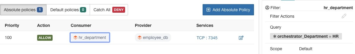
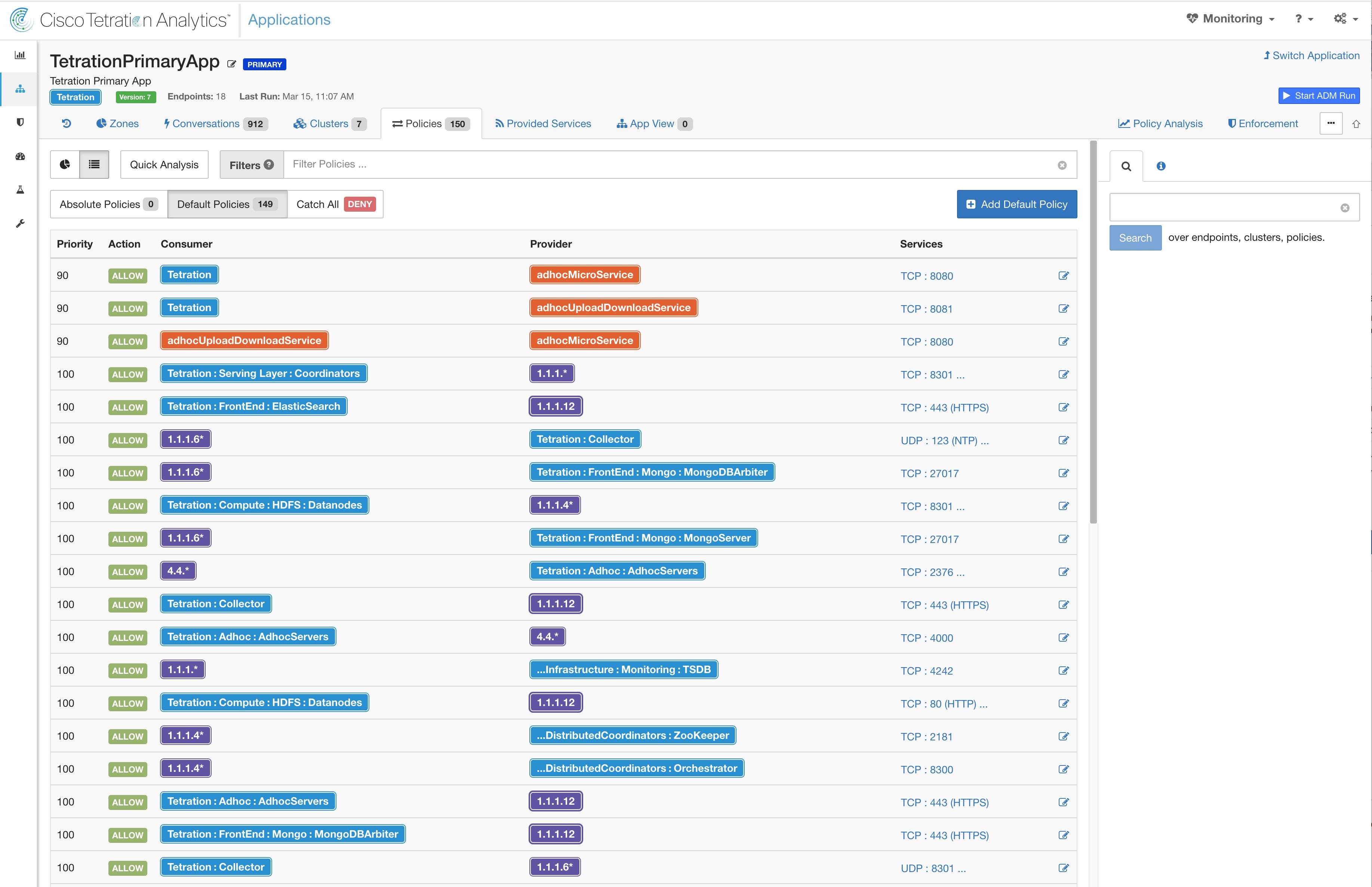
allow traffic from consumer hr_department to provider employee_db

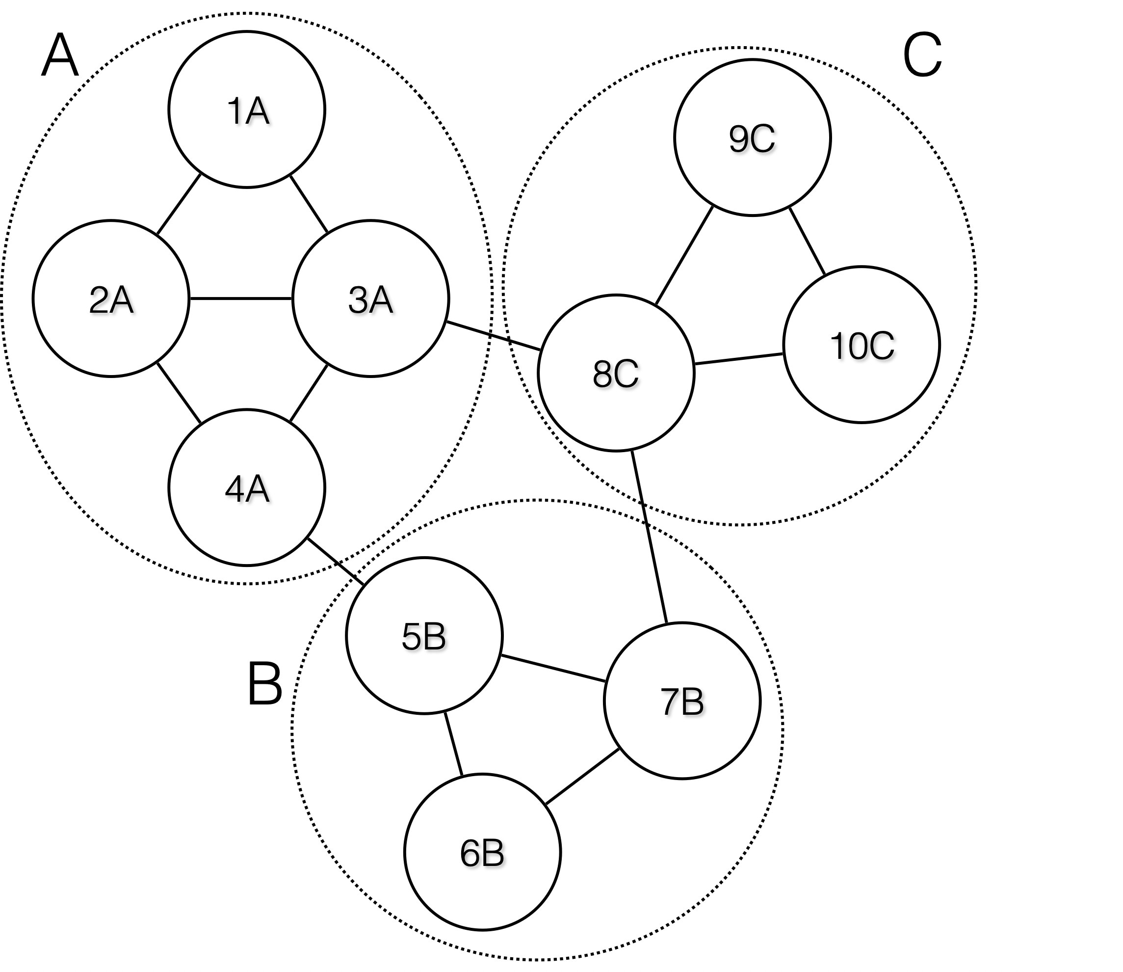
Instead of specifying the members of the consumer and provider workload groups, we can define the logical policy using the labels as shown in the following figure. Note that this allows the membership of the consumer and provider groups to be dynamically modified without the need to modify the logical policy. As workloads are added and removed from the fleet, Secure Workload is notified by services you have configured, such as external orchestrators and cloud connectors. This enables Secure Workload to evaluate the membership of the consumer group hr_department and the provider group employee_db.

Figure 1. Example policy with labels
Example policy with labels

Subnet-based Label Inheritance

Subnet-based label inheritance is supported. The smaller subnets and IP addresses inherit labels from larger subnets they fall under when one of the following conditions is satisfied:

  • The label is missing from the list of labels for the smaller subnet/address.

  • The label value for the smaller subnet/address is empty.

Consider the following example:

IP

Name

Purpose

Environment

Spirit-Animal

10.0.0.1

server-1

webtraffic

production

10.0.0.2

frog

10.0.0.3

eagle

10.0.0.0/24

web-vlan

integration

10.0.0.0/16

webtraffic

badger

10.0.0.0/8

test

bear

The labels for IP address 10.0.0.3 are {“name”: “web-vlan”, “purpose”: “webtraffic”, “environment”: “integra- tion”, “spirit-animal”: “eagle”}.
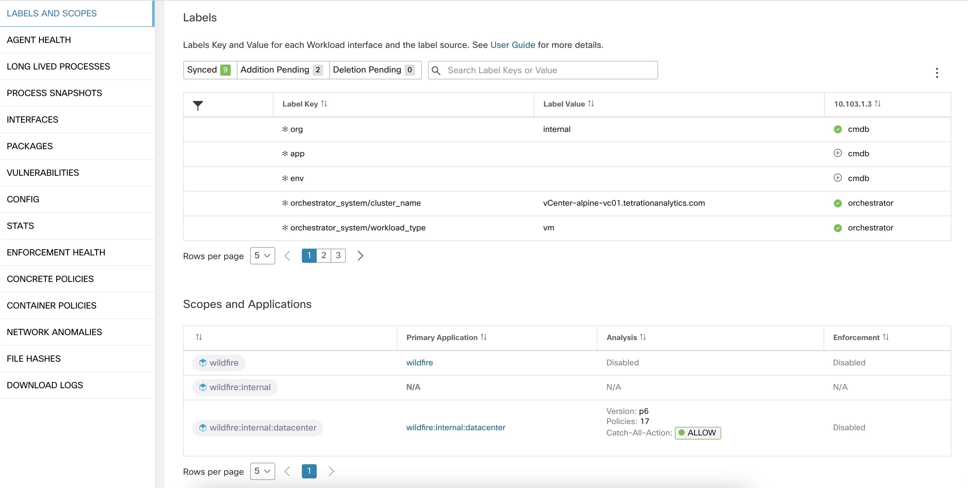
Label Prefixes

Labels are automatically displayed with a prefix that identifies the source of the information.

All user labels are prefixed by * in the UI (user_ in OpenAPI). In addition, labels automatically imported from external orchestrators or from cloud connectors are prefixed with orchestrator_. For labels imported from endpoint connectors, see details in Connectors for Endpoints, but may include labels prefixed with ldap_.

For example, a label with a key of department imported from user-uploaded CSV files appear in the UI as * department, and in OpenAPI as user_department. A label with a key of location imported from an external orchestrator appear in the UI as * orchestrator_location, and in OpenAPI as user_orchestrator_location.

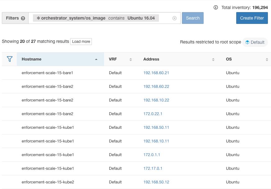
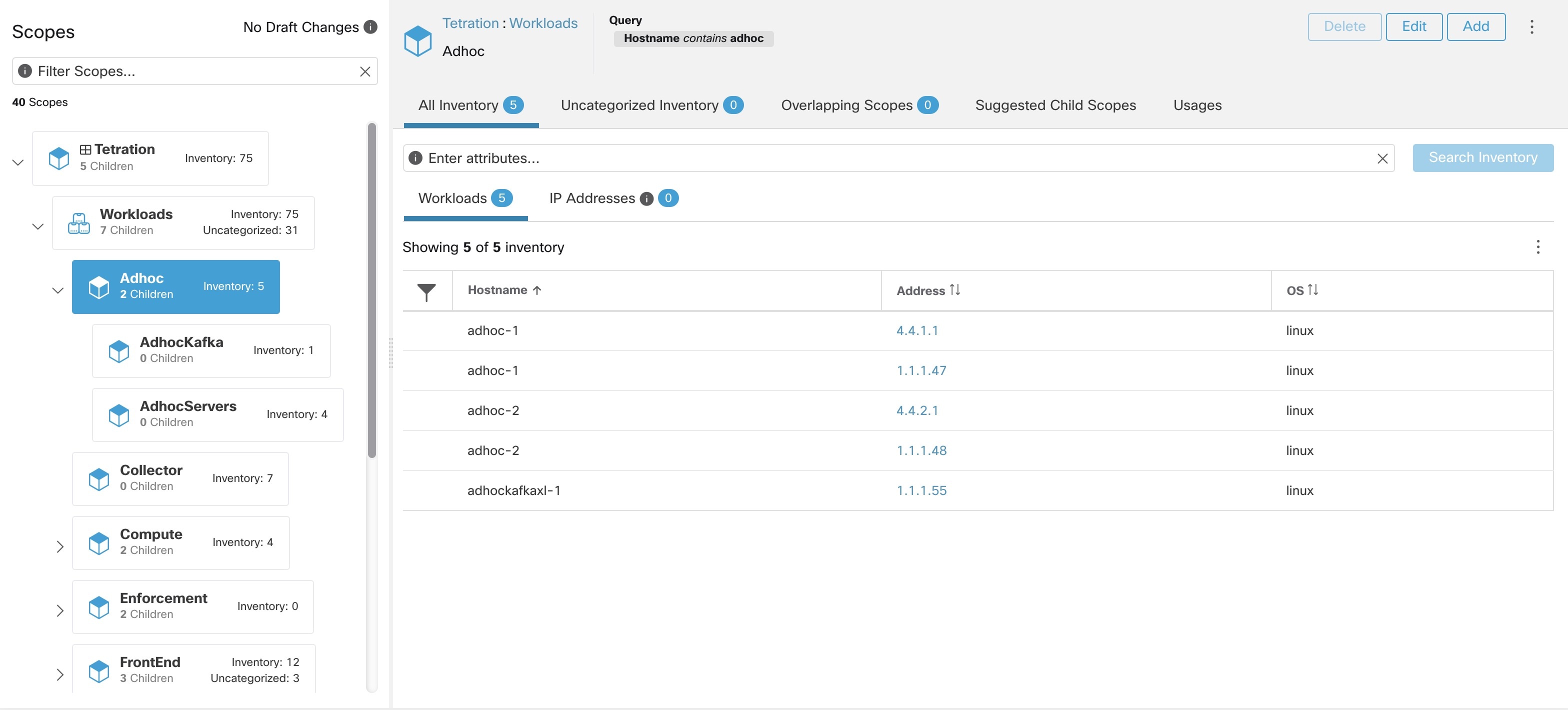
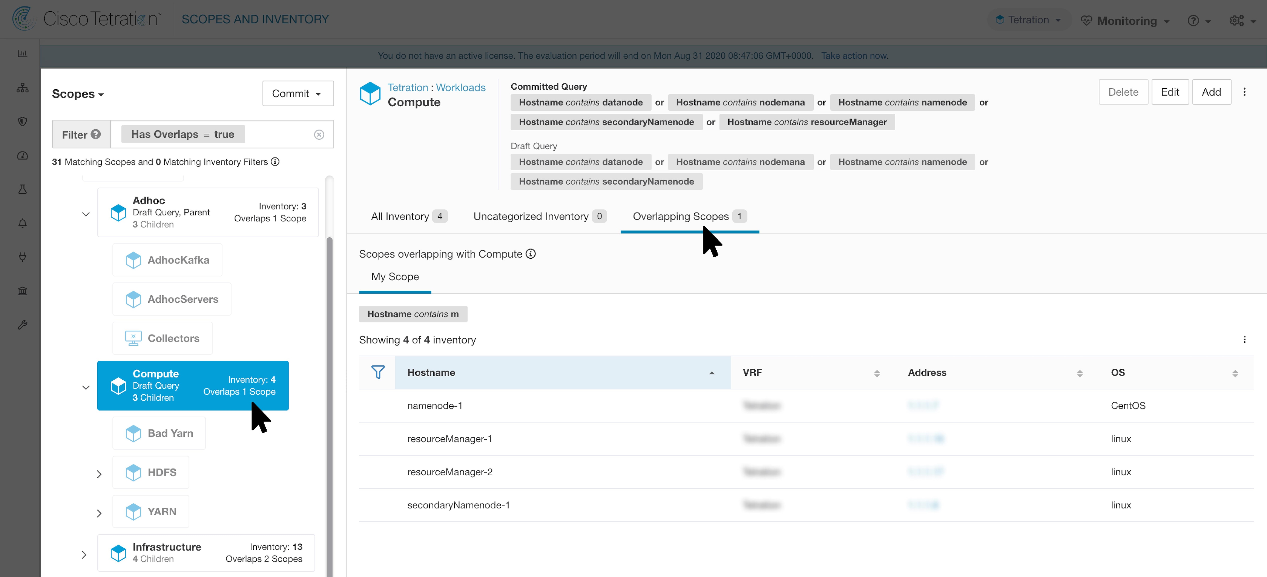
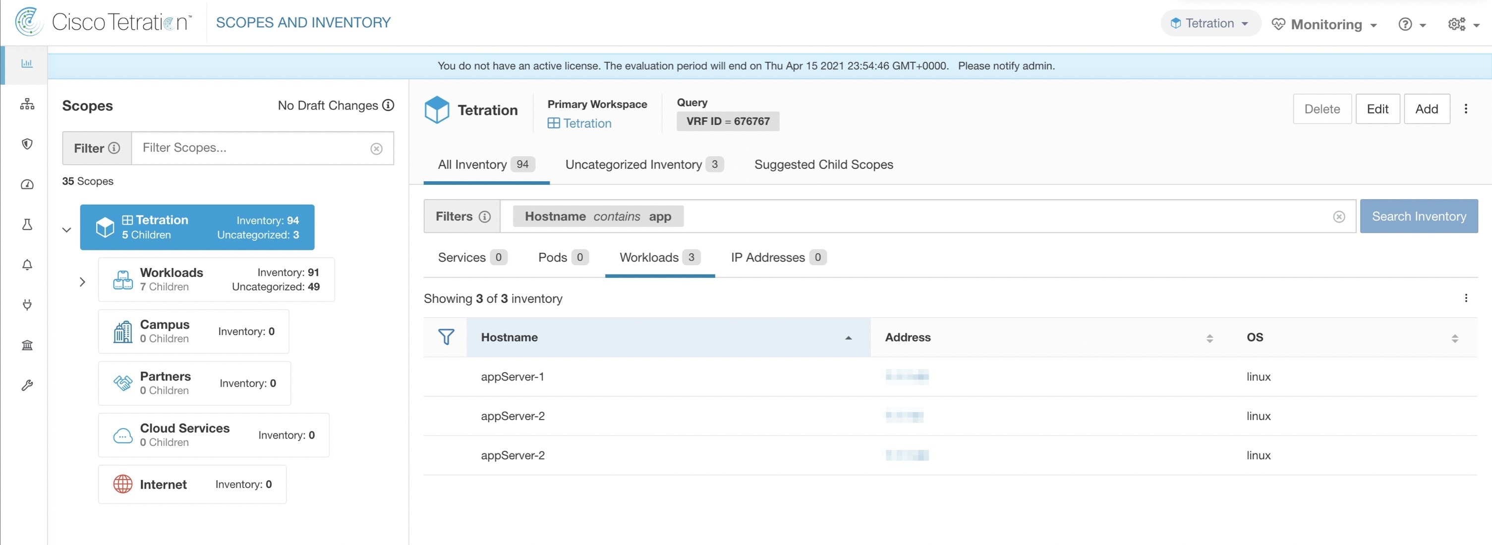
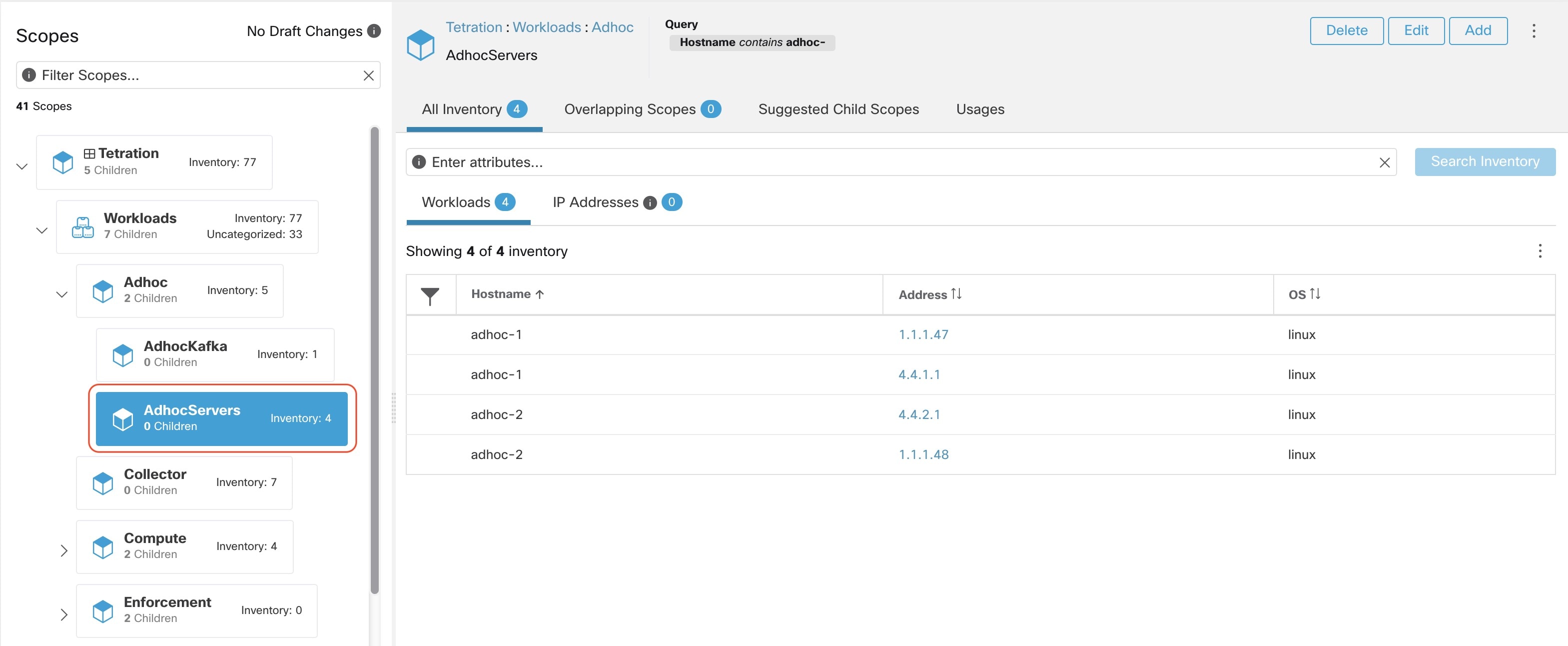
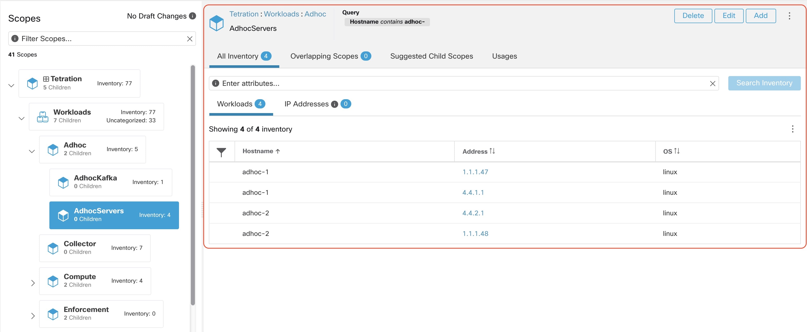
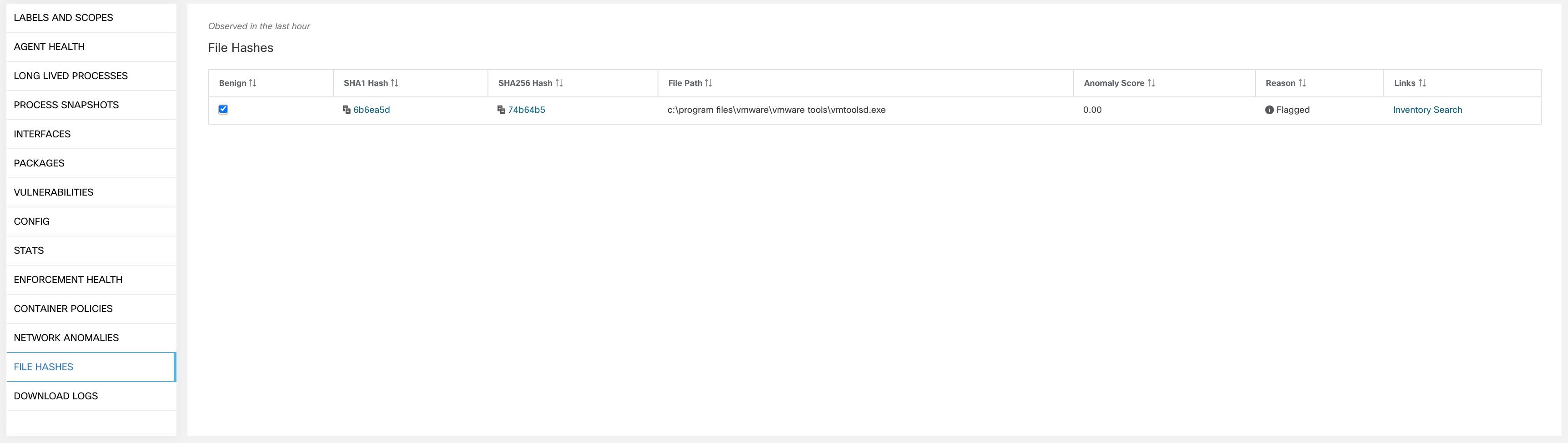
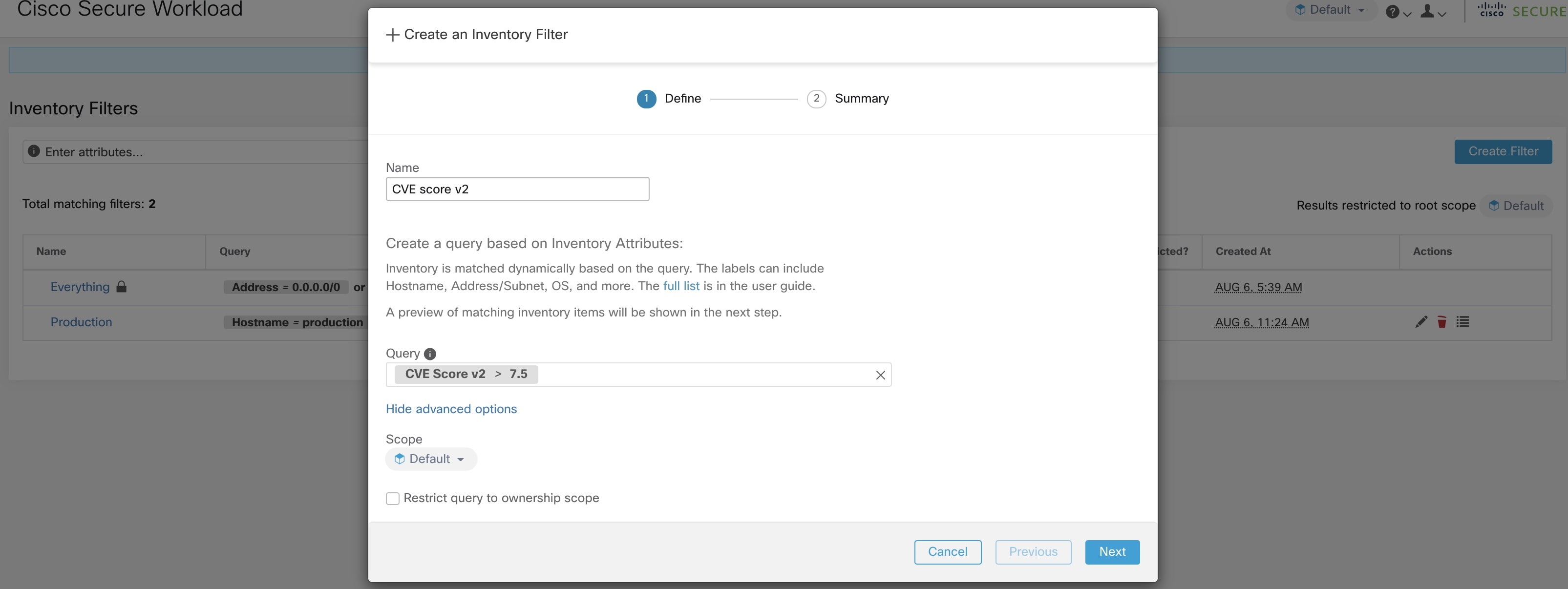
The following figure shows an example of inventory search using the orchestrator-generated label using the prefix:

orchestrator_system/os_image:

Figure 2. Example inventory search with orchestrator generated labels
Example inventory search with orchestrator generated labels

Labels Generated by Cloud Connectors

These labels apply to data from AWS and Azure. The source for these labels is workloads and network interfaces of an AWS VPC or Azure VNet. The tags from the source are merged and displayed in Secure Workload. For example, if the workload tag is
env: prod
and the network interface tag is
env: prod
, the label value in Secure Workload is
prod,test
, which is displayed under the orchestrator_env column on the respective connector page.

For labels specific to AKS, EKS, and GKE, see also Labels Related to Kubernetes Clusters.

Table 1. Labels in Inventory Gathered Using a Cloud Connector

Key

Value

orchestrator_system/orch_type

AWS or Azure

orchestrator_system/cluster_name

<Cluster_name is the name given by the user for this connector’s configuration>

orchestrator_system/name

<Name of connector>

orchestrator_system/cluster_id

<Virtual network ID>

Instance-Specific Labels

The following labels are specific to each node:

Key

Value

orchestrator_system/workload_type

vm

orchestrator_system/machine_id

<InstanceID assigned by the platform>

orchestrator_system/machine_name

<PublicDNS(FQDN) given to this node by AWS> –or– <InstanceName in Azure>

orchestrator_system/segmentation_enabled

<Flag to determine if segmentation is enabled on the inventory>

orchestrator_system/virtual_network_id

<ID of virtual network the inventory belongs to>

orchestrator_system/virtual_network_name

<Name of virtual network the inventory belongs to>

orchestrator_system/interface_id

<Identifier of elastic network interface attached to this inventory>

orchestrator_system/region

<Region the inventory belongs to>

orchestrator_system/resource_group

(This tag applies to Azure inventory only)

orchestrator_‘<Tag Key>‘

<Tag Value> Key-value pair for any number of custom tags assigned to inventory in the cloud portal.

Labels Related to Kubernetes Clusters

The following information applies to plain-vanilla Kubernetes, OpenShift, and to Kubernetes running on supported cloud platforms (EKS, AKS, and GKE).

For each object type, Secure Workload imports inventory live from a Kubernetes cluster, including labels associated with the object. Label keys and values are imported as-is.

In addition to importing the labels defined for the Kubernetes objects, Secure Workload also generates labels that facilitate the use of these objects in inventory filters. These additional labels are especially useful in defining scopes and policies.

Generated labels for all resources

Secure Workload adds the following labels to all the nodes, pods and services retrieved from the Kubernetes/OpenShift/EKS/AKS/GKE API server.

Key

Value

orchestrator_system/orch_type

kubernetes

orchestrator_system/cluster_id

<UUID of the cluster’s configuration in |product|>

orchestrator_system/cluster_name

<Name of kubernetes cluster>

orchestrator_system/namespace

<The Kubernetes/OpenShift/EKS/AKS/GKE namespace of this item>

Node-specific labels

The following labels are generated for nodes only.

Key

Value

orchestrator_system/workload_type

machine

orchestrator_system/machine_id

<UUID assigned by Kubernetes/OpenShift>

orchestrator_system/machine_name

<Name given to this node>

orchestrator_system/kubelet_version

<Version of the kubelet running on this node>

orchestrator_system/container_runtime_version

<The container runtime version running on this node>

Pod-specific labels

The following labels are generated for pods only.

Key

Value

orchestrator_system/workload_type

pod

orchestrator_system/pod_id

<UUID assigned by Kubernetes/OpenShift>

orchestrator_system/pod_name

<Name given to this pod>

orchestrator_system/hostnetwork

<true|false> reflecting whether the pod is running in the host network

orchestrator_system/machine_name

<Name of the node the pod is running on>

orchestrator_system/service_endpoint

[List of service names this pod is providing]

Service-specific labels

The following labels are generated for services only.

Key

Value

orchestrator_system/workload_type

service

orchestrator_system/service_name

<Name given to this service>

  • (For cloud-managed Kubernetes only) Services of ServiceType: LoadBalancer are supported only for gathering metadata, not for collecting flow data or for policy enforcement.


Tip


Filtering items using orchestrator_system/service_name is not the same as using orchestrator_system/service_endpoint.

For example, using the filter orchestrator_system/service_name = web selects all services with the name web while orchestrator_system/service_endpoint = web selects all pods that provide a service with the name web.


Labels Example for Kubernetes Clusters

The following example shows a partial YAML representation of a Kubernetes node and the corresponding labels imported by Secure Workload.


 - apiVersion: v1
 kind: Node
 metadata:
   annotations:
     node.alpha.kubernetes.io/ttl: "0"
     volumes.kubernetes.io/controller-managed-attach-detach: "true"
   labels:
     beta.kubernetes.io/arch: amd64
     beta.kubernetes.io/os: linux
     kubernetes.io/hostname: k8s-controller
Table 2. Label Keys Imported from Kubernetes

Imported label keys

orchestrator_beta.kubernetes.io/arch

orchestrator_beta.kubernetes.io/os

orchestrator_kubernetes.io/hostname

orchestrator_annotation/node.alpha.kubernetes.io/ttl

orchestrator_annotation/volumes.kubernetes.io/controller-managed-attach-detach

orchestrator_system/orch_type

orchestrator_system/cluster_id

orchestrator_system/cluster_name

orchestrator_system/namespace

orchestrator_system/workload_type

orchestrator_system/machine_id

orchestrator_system/machine_name

orchestrator_system/kubelet_version

orchestrator_system/container_runtime_version

Importing Custom Labels

You can upload or manually assign custom labels to associate user-defined data with specific hosts. This user-defined data is used to annotate associated flows and inventory.

There are limits on the number of IPv4/IPv6 addresses/subnets that can be labeled across all root scopes, regardless of label source (whether manually entered or uploaded, ingested using connectors or external orchestrators, and so on) For details, see Label Limits.

Guidelines for Uploading Label Files

Procedure

Step 1

To view a sample file, in the left pane, select Organize > User Uploaded Labels > CSV Upload, and then click Download a Sample.

Step 2

The CSV files used to upload the user labels must include a label key (IP address).

Step 3

To use non-English characters in labels, the CSV file must be in UTF-8 format.

Step 4

Ensure the CSV files meet the guidelines described in the Label Key Schema section.

Step 5

All uploaded files must follow the same schema.


Label Key Schema

Guidelines governing column names
  • There must be one column with a header “IP” in the label key schema. Additionally, there must be at least one other column with attributes for the IP address.

  • The column “VRF” has special significance in the label schema. If provided, it should match the root scope to which you upload the labels. It’s mandatory when uploading the CSV file using the scope independent API.

  • Column names may contain only the following characters: Letters, numbers, space, hyphen, underscore, and slash.

  • Column names cannot exceed 200 characters.

  • Column names cannot be prefixed with “orchestrator_”, “TA_”, “ISE_”, “SNOW_”, nor “LDAP_” since these can conflict with labels from internal applications.

  • The CSV file should not contain duplicate column names.

Guidelines governing column values
  • Values are limited to 255 characters. However, they should be as short as possible while still being clear, distinctive, and meaningful to users.

  • Keys and values are not case sensitive. However, consistency is recommended.

  • Addresses appearing under the “IP” column should conform to the following format:

    • IPv4 addresses can be of the format “x.x.x.x” and “x.x.x.x/32”.

    • IPv4 subnets should be of the format “x.x.x.x/<netmask>”, where netmask is an integer from 0 to 31.

    • IPv6 addresses in the Long format (“x:x:x:x:x:x:x:x” or “x:x:x:x:x:x:x:x/128”) and the Canonical format (“x:x::x” or “x:x::x/128”) are supported.

    • IPv6 subnets in the Long format (“x:x:x:x:x:x:x:x/<netmask>”) and the Canonical format (“x:x::x/<netmask>”) are supported. Netmask must be an integer from 0 to 127.

The order of the columns does not matter. The first 32 user-defined columns will automatically be enabled for label. If more than 32 columns are uploaded, up to 32 can be enabled using the checkboxes on the right-side of the page.

Upload Custom Labels

The following steps explain how users with Site Admin, Customer Support or a root scope owner role can upload labels.

Before you begin

To upload the custom labels, create a CSV file according to the ‘Guidelines for Uploading Label Files’ section.

Procedure

Step 1

In the left pane, select Organize > User Defined Label Upload > CSV Upload, and then under Upload New Labels, click Select File.

Step 2

Select the operation-Add, Merge, or Delete.

  • Add: Appends labels to new and existing addresses/subnets. Resolves conflicts by selecting newer labels over existing ones. For example, if labels for an address in the database are {"foo": "1", "bar": "2"} and the CSV file contains {"z": "1", "bar": "3"}, add` sets labels for this address to {"foo": "1", "z": "1", "bar": "3"}.

  • Merge: Merges labels to existing addresses/subnets. Resolves conflicts by selecting non-empty values over empty values. For example, if labels for an address in the database are {"foo": "1", "bar": "2", "qux": "", "corge": "4"} and the CSV file contains {"z": "1", "bar": "", "qux": "3", "corge": "4-updated"}, merge` sets labels for this address to {"foo": "1", "z": "1", "bar": "2", "qux": "3", "corge": "4-updated"}.

    Note


    Value of “bar” in not reset to “”(empty), instead existing value of “bar”=”2” is preserved.

  • Delete: This option removes labels for an address/subnet, which can significantly impact scopes, filters, policies, and enforced behavior. For important details, see Delete Labels.

Important: The Delete function, while uploading the custom labels, will remove ALL labels associated with the specified IP addresses/subnets, and is not limited to the columns listed in the CSV file. Therefore, the Delete operation must be used with caution.

Step 3

Click Upload.


Search Labels

Users with Site Admin, Customer Support or a root scope owner role can search for, view, and edit labels assigned to an IP address or subnet.

Procedure

Step 1

On the User Uploaded Labels page, click Search and Assign.

Step 2

In the IP or Subnet field, enter the IP address or subnet and click Next.

On the Assign Labels page, the existing labels for the entered IP address or subnet are displayed.


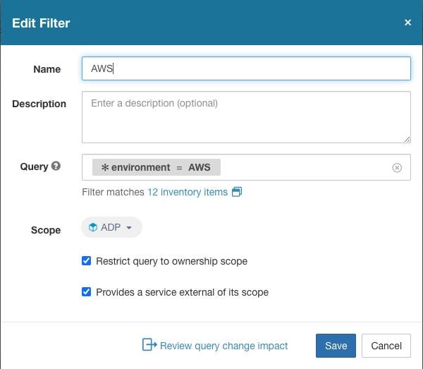
Manually Assign or Edit Custom Labels

Users with Site Admin, Customer Support, or a root scope owner role can manually assign labels to a given IP address or subnet.

Procedure

Step 1

On the User Uploaded Labels page, click Search and Assign.

Step 2

In the IP or Subnet field, enter the IP address or subnet and click Next.

The Assign Labels page is displayed. Note that the existing labels will be displayed and can be edited.

Step 3

To add a new label, in the Labels for <IP address/subnet> section, enter the label name and value, and then click Confirm. Click Next.

Step 4

Review the changes and click Assign to commit them.


Download Labels

Users with Site Admin, Customer Support, or a root scope owner role can download previously defined labels belonging to a root scope.

Procedure

Step 1

On the User Uploaded Labels page, click the CSV Upload tab.

Step 2

Under the Download Existing Labels section, click Download Labels.

The labels used by Secure Workload are downloaded as a CSV file.


Change Labels


Warning


If you need to change a label, do so cautiously, as doing so changes the membership in and effects of existing queries, filters, scopes, clusters, policies, and enforced behavior that are based on that label.


Procedure

Step 1

On the User Uploaded Labels page, click the Search and Assign tab.

Step 2

In the IP or Subnet field, enter the IP address or subnet and click Next.

The labels used by Secure Workload for the entered IP address/subnet are displayed.

Step 3

Under the Actions column, click the Edit icon to change the name and value of the required label.

Step 4

Click Confirm, and then click Next.

Step 5

Review the changes and click Assign.


Disable Labels

One way to change the schema is to disable the labels. Proceed with caution.

Procedure


Step 1

On the User Uploaded Labels page, click the Labels tab.

Step 2

For the required label, under the Actions column, select Disable and confirm to remove the label from the inventory by clicking Yes.

If you decide to enable the label at a later time, click Enable to use the label.


Delete Labels


Warning


One way to change the schema is to disable the labels and delete them. Proceed with caution. This action deletes the selected label which impacts all dependent Filters and Scopes. Ensure that these labels are not used. This action cannot be undone.


Procedure


Step 1

Disable the labels. See disable_lables.

Step 2

Click the TrashCan icon and confirm by clicking Yes to delete the label.
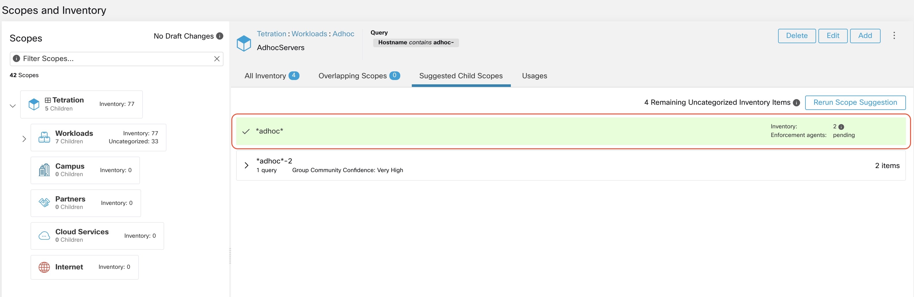
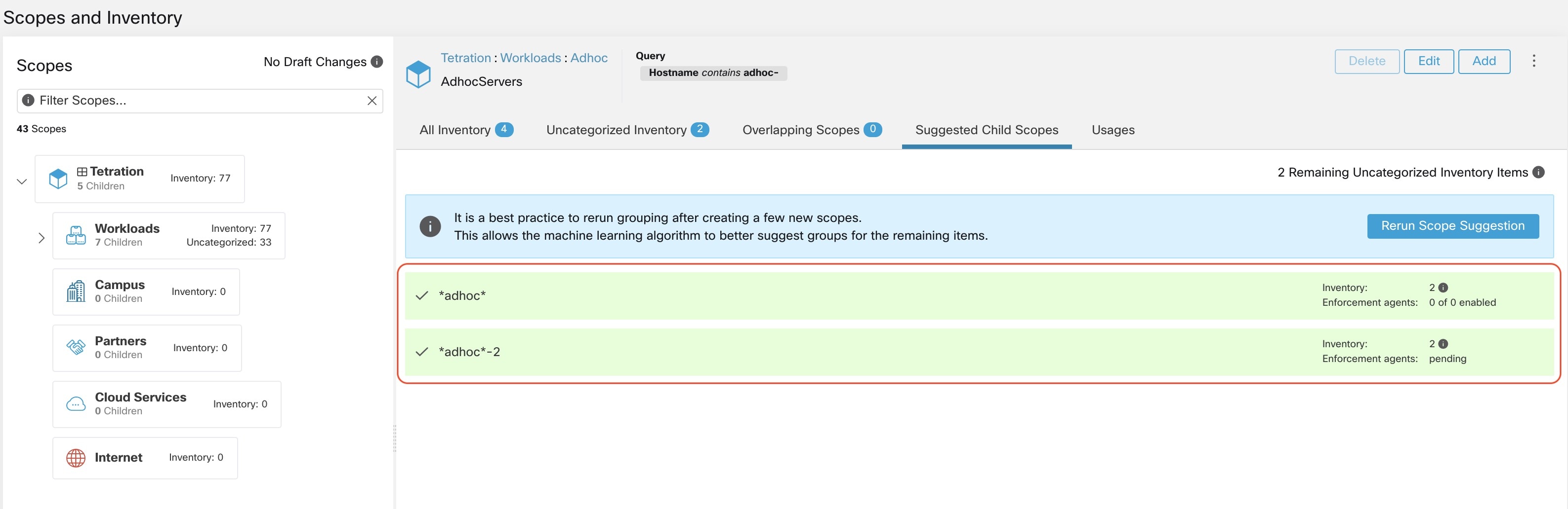
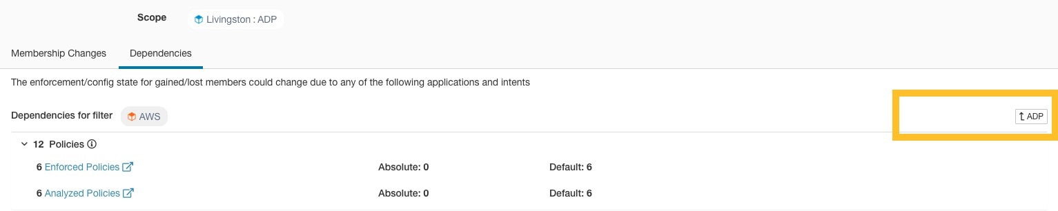

View Labels Usage

The IP addresses/subnet inventory gets updated with the custom labels uploaded using CSV files or manually assigned by users. The labels are then used in defining the scopes and filters, and the application policies are created based on these filters. Therefore, understanding the usage of labels is critical as any modifications to the labels directly impacts the scopes, filters, and policies in Secure Workload.

To view the usage of labels:

Procedure


Step 1

On the User Uploaded Labels page, select the Labels tab. The label keys, top five values of the labels in use, inventory, scopes, filters, and clusters using the custom labels are displayed.
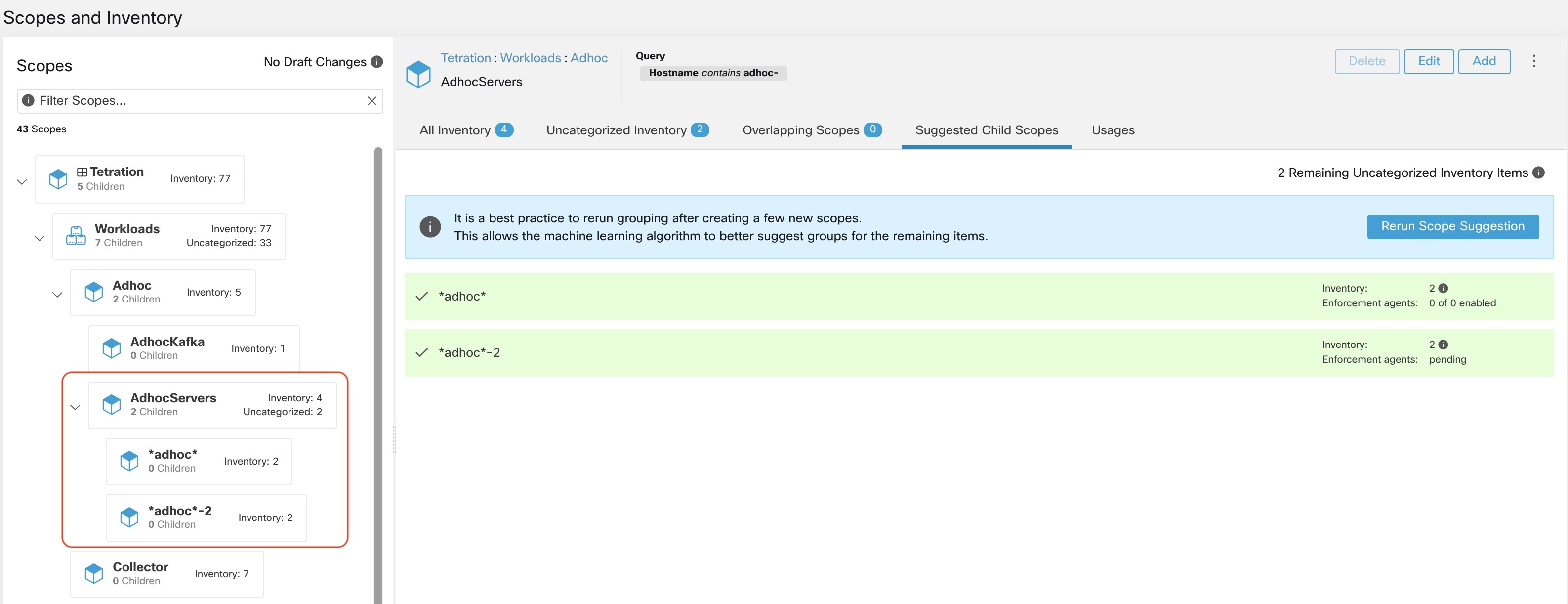
Step 2

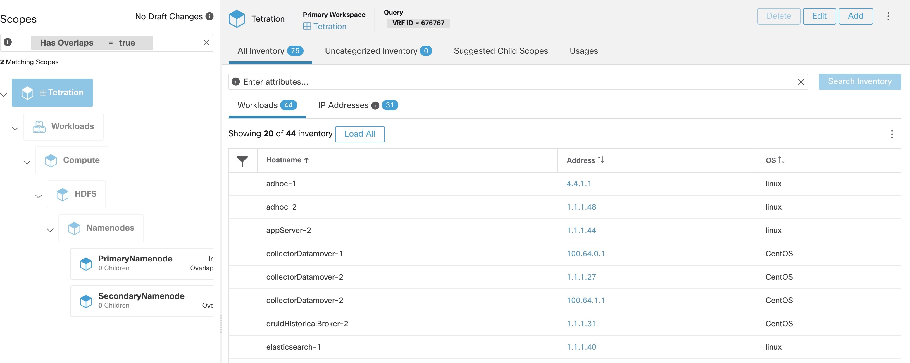
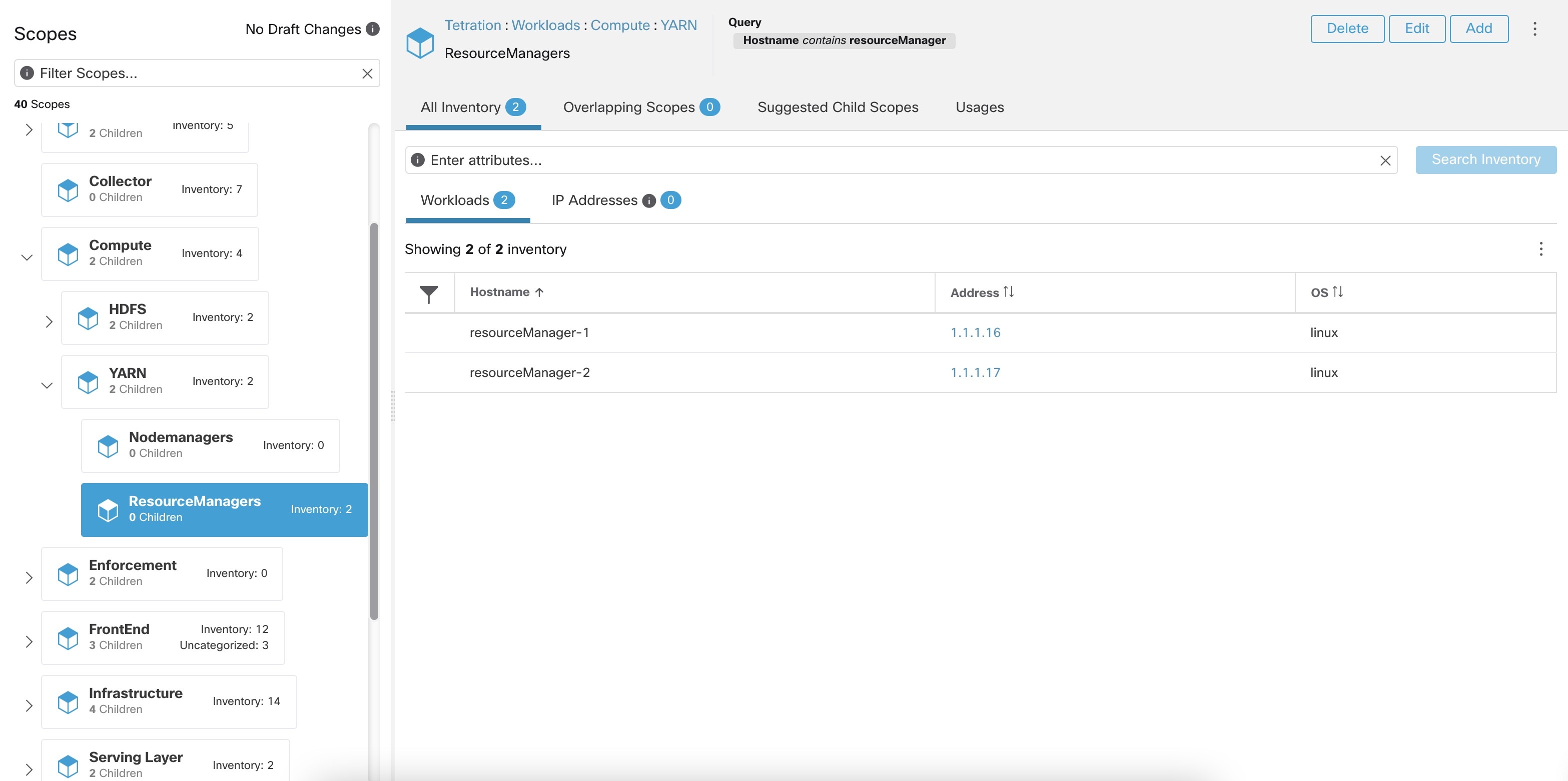
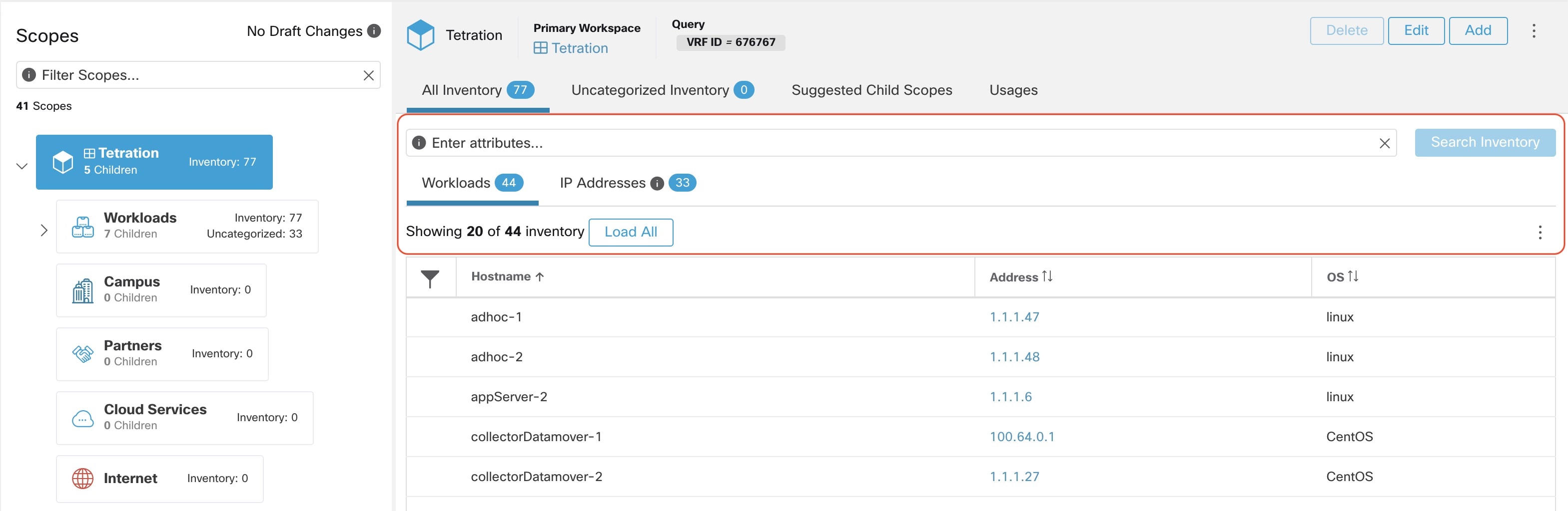
Under the Usages column, click the count values against the inventory, scopes, or filters. For example, to view the scopes using the “Location” label, click the scope queries count.

Figure 3. View scopes of selected label
View scopes of selected label

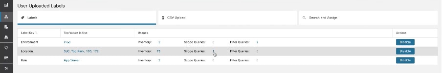
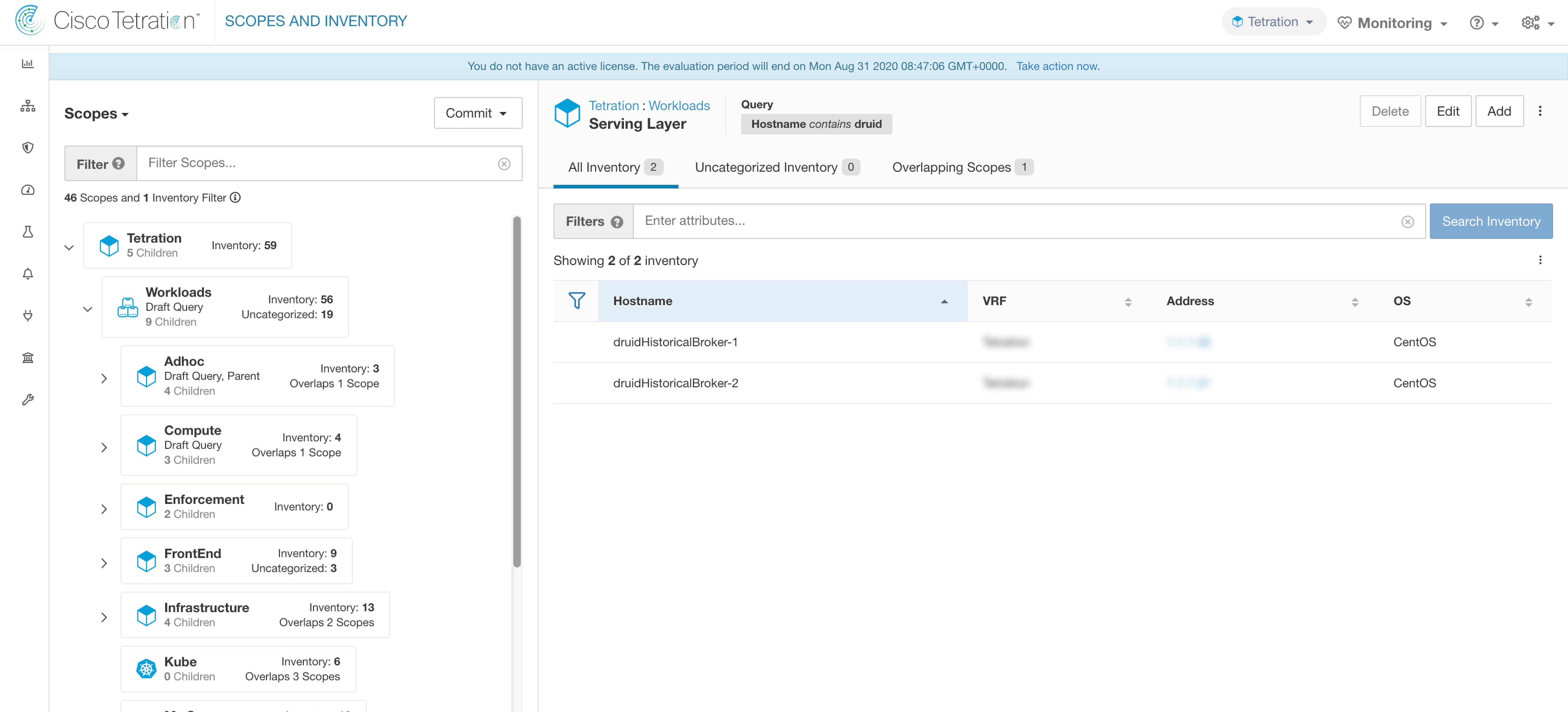
The Scopes and Inventory page is displayed, and the query automatically filters the scopes with the selected label.

Note


You can only view the usage of labels either uploaded using CSV files or those manually assigned to the IP address/subnet.


Create a Process for Maintaining Labels

Your network and inventory will change, and you must plan to update labels to reflect those changes.

For example, if a workload is retired and its IP address is reassigned to a workload with a different purpose, you need to update the labels associated with that workload. This is true for both manually uploaded labels and for labels maintained in and ingested from other systems such as a configuration management database (CMDB.)

Create a process to ensure that your labels are updated on a regular, ongoing basis, and add this process to your network-maintenance routine.

Scopes and Inventory

Scopes and Inventory Overview

This section provides visibility of the scope hierarchy, along with all the inventory it contains. Scopes categorize all of the inventory using a hierarchical structure. See Inventory. On the left is the scope directory user interface. Here, you can traverse down your scope hierarchy. Each scope is displayed in a scope card. It displays the name of the scope, the number of children scopes, the inventory count, and uncategorized inventory if applicable. Clicking on a scope card updates the pane to the right to show details about that scope as well as a filterable list of all its inventory.

Scope Design Principles

  1. Inventory is matched to scope tree according to dynamic query match.

    • Queries may match against IP/Subnet or Label (preferred)

    • Tree is formed through conjunctive query at each layer.

  2. Scope structure may be location specific if appropriate.

    • Combined Cloud vs Data Center and Cloud Specific vs Geographic location

  3. Each layer of the scope tree should represent an anchor point for:

    • Policy control

    • Role Based Access Control (RBAC)

  4. Every child scope should be a subset of its parent scope.


    Note


    Every organization is structured differently, and depending on your industry, require different approaches. Choose one focus in designing your scope hierarchy; location, environment, or application.


    Note


    Do not use IP address or subnet to define scopes that involve Kubernetes inventory. You must use labels to define scopes and policy for these workloads. IP address alone is not sufficient to identify pod services; using IP address for scope definition will produce unreliable results.


Key Features

Filtering feature for both scopes and inventory provides you with the ability to quickly traverse down the scope tree or filter the scope hierarchy and filter the inventory items of the selected scope.

Inventory count is displayed in the scopes card, providing a quick view into the number of workloads in the scope.

Scopes

Scopes are a foundational element to configuration and policy in Secure Workload. Scopes are a collection of workloads arranged in a hierarchy. Workloads labelled to serve as attributes that build a model about where it is, its role, and its function in your environment. Scopes provide a structure to support dynamic mechanisms like identification and attributes associated with an IP that may change over time.

Scopes are used to group datacenter applications and, along with Roles, enable fine grained control of their management. For example, Scopes are used throughout the product to define access to Policies, Flows and Filters.

Scopes are defined hierarchically as sets of trees with the root corresponding to a VRF. As a result, each Scope tree hierarchy represents disjoint data that does not overlap with another Scope tree, see Scope Overlap.

Scope Definition

Each individual Scope is defined with the attributes below:

Attribute

Description

Parent Scope

The parent of the new scope defines the tree hierarchy structure.

Name

The name to identify the scope.

Type

This is used to specify different categories of inventory. If none are applicable, or the scope contains a mix, it can be left blank.

Query

The Query defining the individual scope.


Note


Scopes should be defined in a hierarchy that mimics the application ownership hierarchy of the organization.


Note


Query may match against IP/Subnet or other Inventory attributes.


Figure 4. Example of Traversing through Scope Hierarchy
Example of Traversing through Scope Hierarchy

The scope directory displays the scope hierarchy and some details of each scope (for example, Inventory Count, number of child scopes, Workspaces). Clicking on a scope selects that scope and the details pane to the right updates with more information about that scope and that scope’s inventory.

Figure 5. Inventory count
Inventory count

Scope Filter

Users can use the Scope filter to quickly identify different scope details such as overlapping scopes and query. The filter feature is also helpful in identifying query changes, parent changes, etc.

Field

Description

Name

Filter by the name of the Scope or Inventory Filter.

Description

Filter by text appearing in the description of a scope.

Query

Filter by fields or values used in the query.

Query Change

Filter by scopes that have an uncommitted query.

Parent Change

Filter by scopes that have been moved in the draft but not committed.

Is Inventory Filter

Show Inventory Filters that are restricted to their ownership scope.

Has Workspace

Filter by scopes that have a primary workspace.

Has Enforced Workspace

Filter by scopes that have a primary workspace that is enforced.

Has Overlaps

Filter by scopes that have inventory in common with a sibling scope.

Has Invalid Query

Filter by scopes that have a query that uses invalid or unknown labels.

Examples:

Has Overlaps

Example of Scope Overlap

Figure 6. Has Overlaps
Has Overlaps

For more information see Scope Overlap

Parent Change

Scopes that are moved in the draft but not yet committed.

Figure 7. Parent Change
Parent Change

Full Scope Queries

Figure 8. Example of Scope Hierarchy
Example of Scope Hierarchy

Scopes are defined hierarchically, the full query of the scope is defined as the logical ‘and’ of the scope along with all of its parents. Using the example above, assets assigned to the Workloads:FrontEnd:Mongo

Scope would match:

vrf_id = 676767 and (ip in 1.1.1.0/24) and (Hostname contains mongo).

Where vrf_id = 676767 comes from the root scope query and ip in 1.1.1.0/24 comes from the parent scope query.


Note


It is a best practice to not have overlapping queries at the same level. This removes the importance of ordering and reduces confusion. See Scope Overlap


Providing Access to Scopes

You can grant Read, Write, Execute, Enforce, and Owner abilities on Scopes. An overview is provided below, for more information see Roles.

A User is given access to a “sub-tree”. That is, the given Scope and all its children. Using the preceding example, you have the Read access to the Workloads:FrontEnd scope would, by inheritance, have read access to all the scopes under Workloads:FrontEnd including:

  • Workloads:FrontEnd:Mongo

  • Workloads:FrontEnd:ElasticSearch

  • Workloads:FrontEnd:Redis

  • etc. . .

It’s possible to define Roles with access to multiple Scopes. For example, an “Mongo Admin” role might have Owner access to the Scopes:

  • Workloads:FrontEnd:Mongo:MongoServer

  • Workloads:FrontEnd:Mongo:MongoDBArbiter

Roles and Capabilities allow you to have horizontal access to the Scope hierarchy.

Scope Abilities are also inherited. For example, having the Write ability on a Scope allows one to also Read that information.

Viewing Scope

Every user can view the scope tree they have access to. Users who have the Owner ability on the root scope have the ability to create, edit and delete scope in that tree. To access this view:

In the navigation bar on the left, click Organize > Scopes and Inventory.

You can traverse through the complete scope hierarchy (up to the root) for any Scopes you have access to. This complete traversal provides context as users can create policies to any Scope. Several actions can be performed on this page:

  • Click the chevron in the scope hierarchy to show that scope’s children.

  • Clicking on a scope card will update the pane to the right to show details about that scope as well as a filterable list of all of its inventory.

Figure 9. Example Non-Admin View
Example Non-Admin View

Searching for flows referencing a scope

There are some shortcuts provided on the scopes page to help the user in scenarios they need to search for flows where one or both endpoints of the flow fall within a provided scope.

Figure 10. Searching for flows for a scope
Searching for flows for a scope

After selecting desired scope in the scope tree (left side panel), as shown in the figure above, user can choose between the following three options:

  1. Flow Search - As Consumer provides shortcut to the flow search page to help search for flows with selected scope as Consumer Scope for the flows. In other words, consumer or source endpoint in the flows belongs to the selected scope.

  2. Flow Search - As Provider provides shortcut to the flow search page to help search for flows with selected scope as Provider Scope for the flows. In other words, provider or destination endpoint in the flows belongs to the selected scope.

  3. Flow Search - Internal Traffic provides shortcut to the flow search page to help search for flows that are completely restricted to the selected scope. In other words, both endpoints of the flows (consumer and provider) belong to the selected scope.

Creating a New Scope

Child scopes are created on the Scopes admin page. This action requires the SCOPE_OWNER ability on the root scope. Site Admins are owners of all scopes.

Creating a child scope will impact the application inventory membership (member workloads) of the parent scope. As a result, the parent scope will be marked as having “draft changes”. The changes will need to be committed and dependent structures will need to be updated. See Commit Changes.

Procedure

Step 1

In the navigation bar on the left, click Organize > Scopes and Inventory. The page displays the root Scopes corresponding to Tenants+VRFs already created on the system.

Step 2

Select a child scope in the scope directory. You can filter the scopes first if necessary.

Step 3

Click the Add button.

Figure 11. Scope Add Button
Scope Add Button

Step 4

Enter the appropriate values in the following fields:

Field

Description

Parent

The parent of the new Scope.

Name

The name to identify the Scope. Must be unique under the parent scope

Type

Select a category for the new Scope.

Query

The Query/Filter to match the assets.

Figure 12. Scope Create Modal
Scope Create Modal

Scope Overlap

While adding scopes, it is recommended to avoid overlapping scopes. When scopes overlap, policies generated for overlapping scopes can potentially end up confusing end users. This feature proactively notifies the user if there are any overlapping scope membership, that is, the same inventory belongs to more than one scope at the same depth in scope tree (sibling scopes). The goal is to avoid having the same workload exist in different parts of the scope tree.

To view which inventory items belong to multiple scopes, use the scope filter and enter the Has Overlaps = true facet.

Figure 13. Overlap facet in Scope filter
Overlap facet in Scope filter

The list of overlapping scopes and the corresponding overlapping IP addresses can be viewed by traversing down the scope tree and selecting the Overlapping Scopes tab.

Figure 14. Overlapping Scopes and IPs
Overlapping Scopes and IPs

Editing Scopes

Scopes can only be edited by users with the SCOPE_OWNER ability on the root scope. Site admins are owners of all scopes.

Editing a scope name

Editing a scope name happens immediately and can take several minutes depending on the number of child scopes that need to be updated.


Note


Flow searches by scope name will be impacted when changing the scope name.


Editing a scope query

When a scope’s query is changed the direct parent and child scopes are impacted. Those scopes are marked as having ‘draft changes’ indicating changes have been made to the tree that have not been committed. Once all query updates have been completed, the user must click the Commit Changes button above the Scope Directory to make the change permanent. This will trigger a background task to update all of the scope queries and ‘dynamic cluster queries’ in the workspace.


Warning


Updating a scope query can impact the scopes inventory membership (the workloads that are members of the scope). Changes will take effect during the Commit Changes process. To mitigate risks, you can compare membership changes for further impact analysis from the Review Scope/Filter Change Impact window.

New host firewall rules will be inserted and any existing rules will be deleted on the relevant hosts.


Figure 15. Edit a Scope
Edit a Scope

To edit a scope:

Procedure

Step 1

Click on the edit button on the respective scope to be edited.

Step 2

Edit the Name or Query for the selected scope.

Step 3

Compare changes between the old and new Draft Query by following the Review query change impact link.

Step 4

Click on Save. Name gets updated right away.

Step 5

To update the Query of all scopes, Click the Commit Changes button.

Step 6

You will get a popup confirmation which states the consequences of performing scope changes. The update is processed asynchronously in a background task.

Step 7

Click on Save. Depending on the number of changes this can a minute or more.

Figure 16. Review query change impact
Review query change impact
Figure 17. Commit Changes
Commit Changes

Editing the parent of a scope

When the parent of a scope is updated, the scope query changes. This change effects the membership of both the parent and child scopes. Similar to editing the scope query, these changes are initially saved as ‘draft changes’ and will not go into effect unless they are committed. The user can validate the impact of this change before committing by clicking on “Review query change impact” on the Edit Scope modal. Once validated, the changes can be committed by clicking “Commit” and accepting the “scope moves” and “query changes”.

To edit the parent of a scope:

Procedure

Step 1

Click on the edit button on the respective scope to be edited.

Step 2

Edit the parent for the selected scope.

Step 3

Compare changes between the old and new Draft Query by clicking the Review query change impact link.

Step 4

Click on Save.

Step 5

Click on “Commit” and accept the ‘scope moves’ and ‘query changes’. The update is processed asynchronously in a background task.

Step 6

Depending on the number of workloads this change impacts, this can take a minute or more.

Figure 18. Changing the parent scope from Default scope to Default:ProdHosts
Changing the parent scope from Default scope to Default:ProdHosts

Deleting Scopes

Scopes can only be deleted by users with the SCOPE_OWNER ability on the root scope. Site admins are owners of all scopes.

Deleting a scope will impact the application inventory membership of the parent scope (the workloads that are members of the parent scope). . As a result, the parent scope will be marked as having ‘draft changes’. The changes will need to be committed and dependent structures will need to be updated. See Commit Changes.

Scopes with dependent objects can not be deleted. An error will be returned if:

  • A workspace is defined for the Scope.

  • There is an Inventory Filter assigned to the Scope.

  • A policy exists that uses the Scope to define its consumers or providers.

  • An Agent Config Intent is defined on the Scope

  • An Interface Config Intent is defined on the Scope.

  • A Forensics Config Intent is defined on the Scope.

    To further drill down on scope dependencies, you can visit the Dependencies tab from the Review Scope/Filter Change Impact window.

    These objects need to be removed before the Scope can be deleted.

    1. In the navigation bar on the left, click Organize > Scopes and Inventory.

    2. Select a “scope” then click again to display child Scopes. Select the child scope you wish to delete.

    3. Click the Delete button next to the edit and add buttons.

      Figure 19. Delete Scope
      Delete Scope

      Note


      Only Scopes without children can be deleted


      Note


      Root scopes must be deleted by removing the VRF from the Tenants page.


Reset the Scope Tree

If any of the above configurations exist, you must delete them before you can reset the scope tree. The Reset button is not available until you do so.

To reset the scope tree:

Before you begin

You can delete the entire scope tree and start over.

Resetting the scope tree deletes all scopes, labels, workspaces, and collection rules. It does not delete any ingested data.

Only a user with the SCOPE_OWNER ability on the root scope can reset the scope tree.

However, you cannot reset the scope tree if any of the following are defined for any scope in the tree:

  • Workspaces (except the single workspace created if you created the scope tree using the wizard)

  • Inventory filters

  • Policies

  • Agent Config Intents

  • Interface Config Intents

  • Forensics Config Intents

Procedure

Step 1

From the navigation menu on the left, choose Organize > Scopes and Inventory.

Step 2

Click the scope at the top of the tree.

Step 3

Click Reset.

Step 4

Confirm your choice.

Step 5

If necessary, refresh the browser page to continue.

Figure 20. Reset Scope Tree
Reset Scope Tree

Commit Changes

A scope’s application inventory query definition is defined by its query and those of its direct children. When this happens the scope is marked as having ‘draft changes’ and the scope’s query, workspaces, and clusters will not be changed until the Commit Changes background task is run. When a scope is in draft, the caution triangle is shown by the affected scopes icons, and the ‘Commit Changes’ button is shown on the Scopes page (top right) and should be clicked to run the Commit Changes background task.

Events that can mark a scope as in draft:

  • Query update

  • The query of any parent is updated.

  • Direct child is added.

  • Direct child is deleted.

  • Direct child’s query is updated.

Changing the name of a scope does not change the draft state of the scope.

Figure 21. Commit Changes
Commit Changes

Note


The Commit Changes task is asynchronous. It usually takes several seconds but large scope trees can take several minutes.


Note


The scope update task will be completed when the root scope is no longer in draft. Refresh the page to get the latest state.


Change Log

Site Admins and users with the SCOPE_OWNER ability on the root scope can view the change logs for each scope by clicking change log in the overflow menu in the upper right.

Figure 22. Change Log
Change Log

These users can also view a list of deleted scopes by clicking on the View Deleted Scopes link is in the overflow menu in the upper right corner.

Figure 23. View Deleted Scopes
View Deleted Scopes

Creating a New Tenant

Root level scopes map to VRFs that are created under Tenants or through the Scopes admin page. This action is only available to Site Admins and Customer Support users.

Procedure

Step 1

In the navigation bar on the left, click Platform > Tenants.

Step 2

Click the Create New Tenant button.

Step 3

Enter the appropriate values in the following fields:

Field

Description

Name

The name to identify the Scope. Must be unique under the parent Scope.

Description

An optional description.

Step 4

Click the Create button.

Figure 24. Create Tenant

Inventory

To work with inventory, click Organize > Scopes and Inventory in the left navigation bar.

Inventory Search

All inventory detected on the network is searchable. To search inventory, use the Search Inventory button. Each inventory item is uniquely identifiable by IP and VRF and can be used for performing a search. A service inventory item is not searchable using its IP Address. Use any of the User Labels associated to the service such as user_orchestrator_system/service_name for searching a service inventory. After a host has been found, you can view detailed information about the host on the host profile page.

Inventory Building Blocks

  1. Root Scope

    • Root of the scope hierarchy under a given tenant

    • Provides a logical separation for L3 address domains

  2. Scope

    • Inventory container defined by dynamic query

    • Foundation for hierarchical policy model

    • Anchor point for policy, RBAC, and filter configuration

  3. Filter

    • Flexible construct based on dynamic inventory query

    • Anchor point for intent definition, provided services, and policy definition


    Note


    Includes all IP addresses from partners and anything that is communicating in your environment. Whether they have an agent on them or not, you should define what they are through label.


Label Planning Considerations

  1. Source of data

    • Networks - IPAM? Routing tables? Spreadsheet?

    • Hosts - CMDB, Hypervisor, Cloud, App Owners?

  2. Accuracy of data

  3. How dynamic the data is and how it will be updated.

    • Manual Upload?

    • API Integration?

  4. Start with the basics and grow.

    • Use network labels to build high-level scope structure.

    • Use host labels to build more detailed scope structure at app level.

Searching Inventory

Searching inventory enables you to view information about specific inventory items.

Figure 25. Inventory Search
Inventory Search
Procedure

Step 1

From the top-level menu, select Organize > Scopes and Inventory.

Step 2

Enter the attributes in the Filters field for the inventory item you are looking for. The attributes include the following:

Attributes

Description

Hostname

Enter a full or partial hostname.

VRF Name

Enter a VRF name.

VRF ID

Enter a VRF ID (numeric).

Address

Enter a valid IP address or subnet (IPv4 or IPv6).

Address Type

Enter either IPv4 or IPv6.

OS

Enter an OS name (e.g. CentOS).

OS Version

Enter an OS version (e.g. 6.5).

Interface Name

Enter an interface name (e.g. eth0).

MAC

Enter a MAC address.

In Collection Rules?

Enter true or false.

Process Command Line

Enter the sub-string of a command that is running on host (Note: this facet cannot be saved as part of inventory filter).

Process Binary Hash

Enter the process hash of a command that is running on host (Note: this facet cannot be saved as part of inventory filter).

Package Info

Enter the package name optionally followed by a package version (prefixed by #).

Package CVE

Enter part of or a complete CVE ID.

CVE Score v2

Enter a CVSSv2 (Common Vulnerability Scoring System) score (numeric).

CVE Score v3

Enter a CVSSv3 (Common Vulnerability Scoring System) score (numeric).

User Labels

Attributes prefixed with come from user labels.

Step 3

Click Search Inventory. The results are displayed below the Filters field grouped into four tabs. Each tab displays a table with the relevant columns. Additional columns can be displayed by clicking on the funnel icon in the table header. If any user labels are available, they will be prefixed with and can be toggled here.

Figure 26. Inventory Search Results
Inventory Search Results
Figure 27. Inventory Search Results
Inventory Search Results

The search results are grouped into four tabs:

Tab

Description

Services

Lists the Kubernetes services and load balancers discovered through External Orchestrators. This tab is hidden unless a related external orchestrator is configured.

Pods

Lists the Kubernetes pods. This tab is hidden unless a related external orchestrator is configured.

Workloads

Lists the inventory items reported by Secure Workload agents.

Note


By default, the catch all subnets for IPv4 and IPv6 addresses display in each tenant.

There is also a mention of the inventory count next to each tab. The immediately available information in a search includes hostname, IP Addresses with subnets, OS, OS Version, Service Name and Pod Name. The list of displayed columns can be toggled by clicking the funnel icon in the table header. Search results are restricted to the currently selected scope shown in the scope directory. More information can be seen on the respective profile page by clicking on an item in the search results.

More details about each host is displayed on the Workload Profile, which is accessible by clicking on the IP address field of a search result row. See the Workload Profile for more information.

To create Inventory Filters via the sidebar: Choose Organize > Inventory Filters from the top-level menu. Click on the Create Filter button. A modal dialog appears where you can name your saved filter.


Suggest Child Scopes

Suggest Child Scopes is a tool that uses machine learning algorithms (such as community detection in networks) to discover groupings that could serve as scopes. This tool is helpful when building a scope hierarchy, and facilitates the process of defining more granular child scopes for a given scope. Candidate child scopes are shown as suggestions that can then be selected and added.

Description of Algorithms: A graph based on the communications among the unclaimed members of the parent scope is first created (note: unclaimed members are those that do not belong to any child scope of the parent), and the graph is preprocessed, for example the algorithms attempt to identify endpoints that communicate with sufficiently high proportion of other endpoints in the graph. Such a group of endpoints, if found, is displayed to the user as a candidate common services grouping. The rest of the graph is processed to detect groups that behave as communities, meaning roughly that the endpoints disproportionately communicate with one another more often (or on more provider ports) than to endpoints outside the group. Each such grouping may correspond to an application or a department within the organization. Such a partitioning can also lead to sparser policies among scopes.

Example:

Let 1 through 10 be individual endpoint IPs. Assume the input (communications) graph is as follows:

Figure 28. Input graph
Input graph

Then the endpoints 1 - 4, 5 - 7 and 8 - 10 will be grouped together because they have relatively high degree of communication (number of edges) among one another, and relatively low communications to other endpoints.

Figure 29. Output Groups
Output groups
Steps to perform scope suggestion

To invoke scope suggestion for a desired scope user should locate on the scopes page and select it.

Figure 30. Example of selecting a scope
Example of selecting a scope

In the window, user can browse the inventory, uncategorized inventory items, i.e. those items that belong to the current selected scope and that do not belong to any of the current selected scope’s child scopes. Clicking on the uncategorized inventory items allows one to view this list.

Figure 31. Example of scope window
Example of scope window

After selecting the scope user can click on Suggest Child Scopes, and click on Start Scope Suggestion (or click on Rerun, in case this is not the first time). Note that the input for a scope suggestion run will be the uncategorized inventory items.

Figure 32. Suggest Child Scopes tab
Suggest Child Scopes tab

User can set the date range as input for scope suggestion and click on Suggest Scopes. A scope suggestion run is often fast under medium overall load, and takes only a few minutes for processing ten to thousands of endpoints, with tens of thousands of conversations.

Figure 33. Example of scope suggestion data range selector
Example of scope suggestion data range selector

The output is shown to the user as a list of candidates, currently up to 20 groups (shown), each accompanied with information such as group confidence (quality), a candidate scope name, and queries. Each discovered group has an associated Group Community Confidence, the possible values being: Very High, High, Medium and Low. This is a measure of the Community property of the group: the higher the confidence, the higher the community property of the given group of endpoints (many edges inside the group, relatively few edges to outside). Currently, the subset of groups picked to be shown are selected based on the Group Community Confidence. The groups discovered can currently fall under one of these four group types:

  • Generic Group: Any group discovered via machine learning based on the community property. Note that any group that is not explicitly designated with the special types below is a generic group.

  • Common Service: This group consists of endpoints that communicate with much of the input inventory. These endpoints could be running some kind of shared service(s).

  • Common Service Clients: This group consists of endpoints that only communicate with the Common Service group.

  • Ungrouped: This group consists of endpoints that cannot be grouped since they don’t have sufficient commu- nications.

Figure 34. Example of scope suggestion output
Example of scope suggestion output

The user can click on a discovered group to view the list of queries generated for the selected group. The user can preview the inventory covered by the query which will closely define the discovered group. The queries consist of IP-ranges, subnets, host names and user uploaded labels. There is a confidence measure associated with each group called Query confidence which can have one of the following range of values Perfect, Very High, High, Medium and Low. For query generation, first the groups are discovered via graph processing and machine learning, then the queries are generated for each group. Query Confidence is a measure of how well the query can cover the endpoints. A query confidence of Perfect indicates that the query exactly covers the suggested (discovered) group. On the other end of the spectrum, a Low query confidence indicates that the query significantly misses out on exactly capturing the suggested group, which means that the query covers many Extra IPs (not part of the discovered group) and/or has many Missing IPs (not covered by the query).

Figure 35. Example of scope suggestion output queries
Example of scope suggestion output queries

The user can click on + Scope button which will take the user to an edit window where the user can edit the group name and group query. The user can examine a query, the IPs that it matches, and decide whether some IPs need to be added or removed by adjusting the query. Once satisfied, the user can then click on Next, to review and convert the group to a scope on the draft view canvas.

Figure 36. Example of scope suggestion edit window
Example of scope suggestion edit window

After the user has converted a suggested group to a scope, the group slot turns green and the Uncategorized Inventory Items count decreases.

Figure 37. Example of scope suggestion output after converting one suggested group to a scope
Example of scope suggestion output after converting one suggested group to a scope

The user can repeat the process of scope creation from the remaining list of groups. The recommended workflow is to create one or more scopes and then re-run scope suggestion. A zero count for Uncategorized Inventory Items indicates that there is no inventory left to be further scoped (for the currently selected parent scope).

Figure 38. Example of scope suggestion output after multiple scope creations
Example of scope suggestion output after multiple scope creations

After the scope creation process is done (the uncategorized count is 0), user can repeat this process on the newly created child scopes in order to generate a deeper scope tree as desired.

Figure 39. Example of the scopes list after the initial scope suggestion and creation
Example of the scopes list after the initial scope suggestion and creation

Note


There is also a possibility that the uncategorized items in a scope do not partition well (e.g., do not form communities). In that case, the algorithm may return no groupings (an empty result).


Filters

Filters are saved inventory searches used in defining policies, configuration intents, and so on. Avoid any filter that is associated with a scope, which defines the filter’s ownership scope.

To view existing filters, click Organize > Inventory Filters on the navigation bar. You can also view inventory filters specific to any workspace for any scope.

The list of filters are restricted based on the root of the currently selected scope.

Figure 40. Inventory filters
Inventory filters

You can review inventory membership changes with respect to the selected parent scope by visiting the Review Scope/Filter Change Impact window.

Create an Inventory Filter

Create inventory filters to:

  • Create or discover policies specific to subsets of workloads within a scope.

    For example, create a group of API servers within the scope, the servers must be accessible through the API interface. Create policies to allow only the permissible traffic, but block access to all other workloads for that application.

  • Create policies for workloads that exist across many scopes.

    For example, to create a policy that applies to all workloads on the network running a particular operating system, create an inventory filter that spans across multiple or all scopes.


Tip


To convert an existing cluster to an inventory filter, see Convert a Cluster to an Inventory Filter.


Procedure


Step 1

Navigate to one of the following locations:

  • Choose Organize > Inventory Filters.

  • Navigate to any workspace in a scope for which you want to create an inventory filter and click Manage Policies > Filters > Inventory Filters.

Step 2

Click Create Filter or Add Inventory Filter.

Step 3

Add a name, description, and query that includes all, and only those workloads to include in the filter.

Step 4

Click Show Advanced Options.

Step 5

Specify the scope for the filter.

  • To modify the filter, you must have write access to the specified scope or any of its ancestors.

  • (Depending on other settings in this procedure) The workloads included in the filter.

Step 6

Configure options:

To

Do This

Include workloads that meet the filter query criteria, whether they are members of the scope that is specified in this filter.

Deselect Restrict Query to Ownership Scope

Include only workloads that are members of the scope that is specified in this filter.

Choose Restrict query to ownership scope.

Allow automatic policy discovery to suggest policies specific to the set of workloads defined by this filter.

These workloads must be a subset of the scope that is specified in the filter.

Select Restrict Query to Ownership Scope and Provides a Service External of its Scope.

To use this filter, you must configure external dependencies.

For more information, see Fine-Tune External Dependencies for a Workspace.

Step 7

Click Next.

Step 8

Review the details and click Create.


Restrict to Ownership Scope

Check the Restrict to Ownership Scope? checkbox to determine if the scope impacts the inventory that matches with a filter. For example, in the following structure:

  1. Tenant with query
    VRF ID = 3
  2. Scope within the tenant with the query
    hostname contains db
  3. Inventory filter with the following query that is attached to a scope.
    Platform = Linux
    Figure 41. Tenant, Scope, and Inventory Filter Structure
    Tenant, Scope and Inventory Filter Structure
    • If you do not choose Restrict to Ownership Scope, the filter will match all hosts within the tenant that also matches the filter. Enter the following query:
      (VRF ID = 3) AND (Platform = Linux)
    • If you choose Restrict to Ownership Scope, the filter will match only those hosts within the tenant and the scope that also matches the filter. Enter the following query:
      (VRF ID = 3) AND (hostname contains db) AND (Platform = Linux)

Review Scope/Filter Change Impact

Updating a scope query can impact the scope’s inventory membership after it gets committed. Likewise filter query change, which gets saved directly, can also impact the scope inventory memberships. You can identify membership changes between the new and old queries by following the Review query change impact link on either Scope or Filter Edit modals. In addition, knowing the scope or filter dependencies can be helpful for impact analysis and removing all necessary objects preventing Scope deletion. Visit the Dependencies tab as well, to traverse the Scope Dependencies tree for further information.

Figure 42. Download Membership Table
Download Membership Table

Scope Query Change Impact Modal

Both Membership Changes and Dependencies tab can be accessed by following the link to Review query change impact on Scope Edit window.

Membership Changes

The inventory table under Membership view displays all columns by default. You can choose the columns to display. Furthermore, you can download the csv or json of chosen Membership columns and rows with an additional Diff column identifying whether the inventory is Gained, Lost or Unchanged. Be sure that all table selection desired for download is visible to the table view.

Figure 43. Scope Membership Changes
Scope Membership Changes

Dependencies

You can traverse down to nested dependencies by further selecting Review Dependencies

Figure 44. Review Dependencies
Review Dependencies

You can traverse back up the dependencies tree by selecting the selected Parent link:

Figure 45. Parent Link
Parent Link

The following are Scope Dependencies which may exist:

Table 3. The following are Scope Dependencies which may exist

Type

Description

Application

Has primary and secondary application names and links to the specific workspaces under Segmentation.

Child Scopes

Has names and links to child Scope Detail views. Allows drill down to lower level Dependencies.

Policies

Has analyzed and enforced policies counts and links to respective Global Policy Views filtered by selected scope.

Restricted Inventory Filters

Has names and links to child Filter Detail views. Allows drill down to lower level Dependencies.

Config Intents

Has names and links to Agent, Interface and Forensics Config Intents views.

Filter Query Change Impact Modal

Both Membership Changes and Dependencies tab can be accessed by following the link to Review query change impact on Inventory Filter Edit window.

Membership Changes

Figure 46. Inventory Filter Membership Changes
Inventory Filter Membership Changes

Dependencies

The following are Filter Dependencies which may exist:

Type

Description

Policies

Has analyzed and enforced policies counts and links to respective Global Policy Views filtered by selected scope

Config Intents

Has names and links to Agent, Interface and Forensics Config Intents views

Inventory Profile


Note


An inventory profile page is linked from various places. One of the ways to see an inventory profile is to perform a search for inventory, then click an IP address to go to its profile. If you are working in the Scopes and Inventory page, click an IP address in the IP addresses tab, not an IP address in the Workloads tab. (Clicking an IP address in the Workloads tab displays the Workload Profile, not the Inventory Profile.)


The following information is available for the inventory:

Field

Description

Scopes

List of scopes that the inventory belongs to.

Inventory Type

  • Flow Learnt inventory was registered based on the observed flows.

  • Labeled inventory was manually uploaded using the inventory upload utility.

  • Agent inventory was reported by the software agent installed on a host.

  • Tagged inventory was either reported by connectors or external orchestrators.

User Labels

The list of user uploaded attributes for this inventory. See User Labels for more details.

Additional information is available only if both of the following are true:

  1. Inventory has been ingested through a cloud connector.

  2. Segmentation is enabled for the virtual network in which the inventory resides.

    Field

    Description

    Enforcement Health

    The status information of the host software agent. See Agent Health Tab for more details.

    Concrete Policies

    This tab shows Secure Workload concrete enforcement policies applied on the host. See Concrete Policies Tab for more details.

    Security Groups

    The list of security groups and their policies applied to this inventory.

Inventory Profile Information

Field

Description

Experimental Groups

A list of cluster or user-defined inventory filters that are used for policy live analysis.

Enforcement Groups

A list of cluster or user-defined inventory filters that are used for policy enforcement. They can be different from experimental groups depending on the versions of policies being analyzed and/or enforced in the system.


Note


The inventory profile details may not be available for an IP address when:

  • The inventory is excluded from collection rules.

  • In a unidirectional flow, the inventory is available only for two minutes, and then it is removed.

  • In a bidirectional flow, the inventory is available for 30 days. If no more flows are observed during these 30 days then the inventory details are removed.


Workload Profile

Workload profile displays detailed information about a host where Secure Workload software agent is installed. This section explains how to view a workload profile and the information it contains.


Note


A workload profile page is linked from various places. One of the ways to see a workload profile is to perform a search for host as described in search


From the results of inventory search, click on IP address of the host to go to it’s profile. Based on the type of agent installed on the host, the following tabs are available on the page. Note that you may end up on inventory profile page if Secure Workload software agent is not installed on the host that this inventory belongs to.

Labels and Scopes Tab

This tab includes the enforcement and experimental groups, scopes that the host belongs to. The experimental groups are inventory filters that are used for policy live analysis, while the enforcement groups are the filters that are used for policy enforcement. They can be different depending on the versions of policies being analyzed and/or enforced in the system.

Figure 47. Workload Labels and Scopes
Workload Labels and Scopes

Agent Health Tab

The status information of the host software agent such as it’s type, OS platform, agent version and last check-in time are also shown in the Agent Health tab. See Software Agent Config for more details. This tab also shows detailed time series data for traffic bytes and packets occurred per one day.

Figure 48. Workload Agent Health Details
Workload Agent Health Details

For users with root scope owner privileges, summary page also includes a section to collect and download agent logs for deep visibility and enforcement agents (versions 3.3 or later) within that root scope. Also note that this feature is not available for agents running on platforms AIX and SUSE Linux Enterprise Server (s390x-Linux on IBM Z architectures). Use “Initiate Log Collection” button to collect logs from the agent and then logs are available for download in a few minutes. If the download fails, retry collection of logs, and then attempt download again.

Figure 49. Agent Logs
Agent Logs

Process List Tab

This tab shows list of processes running on the host. A filter is also available to narrow down the list of processes based on the attributes of a process shown in table header below.

Figure 50. Workload Process List
Workload Process List

Attribute Descriptions:

Attribute

Description

Last Exec Content Change

Similar to mtime in linux. It is the timestamp when only the file content changes.

Last Exec Content Change

Similar to ctime in linux. It is the timestamp when either the file content or attribute changes.

Last Seen

Last time when the process is observed. Available when the process is dead.

CPU Usage

CPU usage trend by the process in the past hour.

Memory

Usage

Memory usage trend by the process in the past hour.

Process Binary Hash

SHA256 hash of the process binary in hex string, also known as process hash for short. Not available for kernel processes.

Anomaly Score

Process hash (anomaly) score. See Process hash anomaly detection for more information.

Verdict

Verdict of the process hash (either Malicious or Benign). The verdict is determined based on whether the process hash belongs to any user-defined hash list or known threat-intelligence hash database. See Process hash anomaly detection for more information.

Verdict Source

Source of the verdict. The verdict source can be either User Defined, or Secure Workload Cloud, or NIST. This attribute is known as Hash DB Source in previous releases. See Process hash anomaly detection for more information.

Process Snapshot Tab

This tab shows searchable process tree observed on the workload.

Figure 51. Workload Process Snapshot
Workload Process Snapshot

Interfaces Tab

This tab shows details about the network interfaces installed on the host. It's available for all types of software agents.

Figure 52. Workload Interface List
Workload Interface List

Software Packages Tab

This tab shows the list of packages installed on the host. You can selectively view software packages based on package attributes in the table header.

Figure 53. Software Packages List
Software Packages List

Vulnerabilities Tab

This tab shows searchable vulnerabilities observed on the workload based on the Common Vulnerabilities and Exposures (CVE) system. See Vulnerability data visibility

Figure 54. Vulnerabilities Tab
Vulnerabilities Tab

Agent Configuration Tab

This tab shows software agent settings. It is only available for Deep Visibility and Enforcement Agents. These settings can be modified using Agent Configuration Intents via the agent config page. See Software Agent Config

Figure 55. Applied Workload Configuration
Applied Workload Configuration

Agent Statistics Tab

This tab shows statistics about the Secure Workload agent installed on the host. It's only available for Deep Visibility and Enforcement Agents.

Figure 56. Agent Statistics
Agent Statistics

Concrete Policies Tab

When a workspace is enforced, each workload receives only the policies in that workspace that are specific to that workload. These policies that are actually programmed on each workload are called concrete policies.

For example, suppose the provider specified in a policy with action ALLOW includes all inventory in the subnet 1.1.1.0/24. When this policy is installed on a workload with a Secure Workload agent and having IP address 1.1.1.2, the firewall rules look like this:

  1. For incoming traffic firewall rules allow traffic destined to 1.1.1.2 specifically, not to the whole subnet 1.1.1.0/24.

  2. For outgoing traffic firewall rules allow traffic sourced from 1.1.1.2 specifically, not from the whole subnet 1.1.1.0/24.

The CONCRETE POLICIES tab in the Workload Profile shows Secure Workload concrete enforcement policies applied on the host. Each row in this table corresponds to a firewall rule implemented on the host. Each policy row can be further expanded to display the logical intent from which this concrete policy derived. Packet and byte count time series view is also available for each rule. Click the Fetch All Stats button to view packets and bytes count for each rule. A filter is also available in this tab to narrow the list of enforced policies based on attributes of a policy shown in table header below. This tab is only available when the installed agent is enabled for enforccement.

Figure 57. Concrete Policy List

In the image below, Policy Groups shows the consumer and provider:

Figure 58. Concrete Policy Row
Concrete Policy Row

Container Policies Tab

This tab shows Secure Workload concrete enforcement policies applied on the containers. Each row in this table corresponds to a firewall rule implemented on the container pod.

Figure 59. Container Concrete Policy List
Container Concrete Policy List

Network Anomalies Tab

This tab helps to identify the events with large data movements in or out of this workload. See PCR-based Network Anomaly detection for more information.

Figure 60. Workload Network Anomalies
Workload Network Anomalies

File Hashes Tab

This tab detects process hash anomalies by assessing the consistency of process binary hashes across the system. See Process hash anomaly detection for more info.

Figure 61. Workload File Hashes
Workload File Hashes

Software Packages

The Software Packages feature set allows viewing packages installed on hosts and the vulnerabilities affecting them. Specifically, it allows to:

  • View packages registered with the following package managers:

    • Linux: Redhat Package Manager (RPM) and Debian Package Manager (dpkg)

    • Windows: Windows Registry Service

  • View Common Vulnerabilities and Exposures (CVEs) affecting packages installed on a host.

  • Define inventory filters using the package name and version.

Packages Tab

To view packages installed on a host, navigate to the packages tab on the workload profile Workload Profile page.

Figure 62. Workload profile packages
Workload profile packages

Common Vulnerabilities and Exposures (CVEs)

In addition to displaying packages under the packages tab, we display common vulnerabilities affecting them along with their severity. Each vulnerability contains a link to the Nation Vulnerability Database (NVD) which provides more information on the specific vulnerability. In addition to displaying the CVE ID, we also display the impact score (on a scale of 10), indicative of the severity of the vulnerability.

Figure 63. Workload profile packages CVE
Workload profile packages CVE

Windows Packages and CVEs

Following section lists the behavior of Windows agent with regard to reporting package information to Secure Workload.

  • Windows applications, PowerShell, IE are reported as packages. .net framework is also reported as a package.

  • Other Windows applications like notepad.exe, cmd.exe, mstsc.exe, and so on are not reported.

  • Windows server configured roles and features are reported as packages but the version may be incorrect. For example: If the DNS server is configured, reported version will either 0 or 8.

  • Windows agent reports 3rd party products installed using MSI installer or exe installer:

    • For MSI installers, MSI APIs are used to retrieve package information. For example, version, publisher, package name.

    • If the exe installer is used to install the package, package information is retrieved from the registry.

    • Package installer fields like version, publisher is optional. If version is missing, the package will not be reported.

    • If a product is extracted from zip file or installed as an app, it will not be reported in the package list.

Inventory Filters

Package related information can be searched by defining an inventory filter with the package name and version (optional).

The syntax for this filter is as follows: PackageName#PackageVersion

Figure 64. Inventory package

The following operations are supported:

  • Equality - returns hosts with packages matching PackageName and the PackageVersion (if provided).

  • Inequality - returns hosts with packages matching PackageName but not the PackageVersion (if provided).

  • Greater Than - returns hosts with packages matching PackageName and with version greater than PackageVersion.

  • Greater Than or Equal To - returns hosts with packages matching PackageName and with version greater than or equal to PackageVersion.

  • Less Than - returns hosts with packages matching PackageName and with version less than PackageVersion.

  • Less Than or Equal To - returns hosts with packages matching PackageName and with version less than or equal to PackageVersion.

Vulnerability data visibility

The Vulnerability data visibility feature allows for detecting and viewing vulnerabilities affecting packages and processes on a host. Inventory filters can be defined using:

- CVE IDs.- CVSS v2 and v3 scores.- CVSS v2 access vector and access complexity.- CVSS v3 attack vector, attack complexity, and privilege required.

Workload Profile Page

Vulnerability related information affecting packages and processes on a system is displayed on the Workload Profile page.

Packages Tab

The packages tab lists packages installed on a host and vulnerabilities affecting them.

Figure 65. Workload profile packages
Workload profile packages

Process List Tab

Long-lived processes are displayed under the process list tab.

Figure 66. Workload profile process list
Workload profile process list

Process Snapshot Tab

Vulnerability information is displayed for all processes in the process tree under the process snapshot tab.

Figure 67. Workload profile process snapshot tab
Workload profile process snapshot tab

Vulnerabilities Tab

The vulnerability tab shows a list of vulnerabilities observed on the workload.

For each CVE, besides basic impact metrics, exploit information based on our threat intelligence is displayed:

  • Exploit Count: number of times CVE was seen exploited in the wild in the last year

  • Last Exploited: last time CVE was seen exploited in the wild by our threat intelligence

Figure 68. Workload profile vulnerabilities tab
Workload profile vulnerabilities tab

Inventory Filters

The following types of inventory filters can be defined to identify hosts with vulnerable packages:

CVE ID based filter

This filter allows searching for hosts affected by a specific CVE or any CVE.

To search for a host affected by a specific CVE, provide the CVE ID in the format: CVE-XXXX-XXXX

Figure 69. Inventory filter CVE
Inventory filter CVE

The following operations are supported:

  • Equality - returns hosts with packages affected by a CVE ID.

  • Inequality - returns hosts with packages not affected by a CVE ID.

  • Contains - returns hosts with packages affected by a CVE present in the input string (entering “cve” will return hosts affected by a CVE).

  • Doesn’t contain - returns hosts with packages not affected by a CVE present in the input string (entering “cve” will return hosts not affected by a CVE).

CVSS (Common Vulnerability Scoring System) impact score based filter

This filter allows searching for hosts that have CVE with the specified CVSSv2 or CVSSv3 impact score. To search for hosts which have any CVE with impact score (v2 or v3), user can provide the score in numeric format.

To search for hosts which have CVE with CVSSv2 impact score greater than 7.5.

Figure 70. Inventory filter CVSS
Inventory filter CVSS

The following operations are supported:

  • Equality - returns hosts which have CVE with the specified CVSSv2 or CVSSv3 impact scores.

  • Inequality - returns hosts which don’t have CVE with the specified CVSSv2 or CVSSv3 impact scores.

  • Greater Than - returns hosts which have CVE with CVSSv2 or CVSSv3 impact scores greater than the specified CVSSv2 or CVSSv3 impact scores respectively.

  • Greater Than or Equal To - returns hosts which have CVE with CVSSv2 or CVSSv3 impact scores greater than or equal to the specified CVSSv2 or CVSSv3 impact scores respectively.

  • Less Than - returns hosts which have CVE with CVSSv2 or CVSSv3 impact scores less than the specified CVSSv2 or CVSSv3 impact scores respectively.

  • Less Than or Equal To - returns hosts which have CVE with CVSSv2 or CVSSv3 impact scores less than or equal to the specified CVSSv2 or CVSSv3 impact scores respectively.

CVSSv2 based filters

Inventory filters can be created using access vectors and access complexities to identify vulnerable hosts. These filters support the following types of operations:

  • Equality - returns hosts with packages affected by vulnerabilities matching the filter.

  • Inequality - returns hosts with packages not affected by vulnerabilities matching the filter.

Access Vector

Access vector reflects how the vulnerability is exploited. The farther the attacker can get from the vulnerable system, the higher the base score. The table below lists different access vectors with their access requirements:

Value

Type of access

LOCAL

Physical or local (shell).

ADJACENT_NETWORK

Broadcast or collision.

NETWORK

Remotely exploitable.

Access Complexity

This metric measures the complexity in exploiting a vulnerability once the attacker is able to access the target system. The base score is inversely proportional to the access complexity. The different types of access complexities are as follows:

Value

Description

HIGH

Specialized access conditions exist.

MEDIUM

Access conditions are somewhat specialized.

LOW

Specialized access conditions do not exist.

CVSSv3 based filters

Attack vectors, attack complexities, and privilege required to influence the CVSSv3 score and can be used in inventory filters. These filters support the following operations:

  • Equality - returns hosts with packages affected by vulnerabilities matching the filter.

  • Inequality - returns hosts with packages not affected by vulnerabilities matching the filter.

Attack Vector

This metric reflects the context by which vulnerability exploitation is possible. The farther an attacker can get from the vulnerable component, the higher the base score. The table below lists different attack vectors with their access requirements:

Value

Type of access

LOCAL

Local (keyboard, console) or remote (SSH).

PHYSICAL

Physical access is needed.

ADJACENT_NETWORK

Broadcast or collision.

NETWORK

Remotely exploitable.

Attack Complexity

This metric describes the conditions that must exist in order to exploit the vulnerability. The base score is greatest for least complex attacks. The different types of access complexities are as follows:

Value

Description

HIGH

Significant effort needed in setting up and executing the attack.

LOW

Specialized access conditions do not exist.

Privileges Required

This metric describes the level of privileges an attacker must possess before successfully exploiting the vulnerability. The base score is highest when privileges aren’t needed to carry out an attack. The different values of privilege required are as follows:

Value

Privileges required

HIGH

Privileges providing significant control over the vulnerable component.

LOW

Low privileges that grant access to non-sensitive resources.

NONE

Privileges aren’t needed to carry out an attack.

Service Profile

Secure Workload provides visibility of all Kubernetes services and other Load Balancers ingested through an external orchestrator. Service profile page shows the details for a given service.


Note


Service profile page is linked from various places. One of the ways to see a service profile is to perform a search for service as described in search


From the results of search, click on a Service Name under the Services tab to go to its profile. The following information is available for the service:

Header

Header consists of:

  • Orchestrator Name: Name of the external orchestrator which reported this service.

  • Orchestrator Type: Type of the external orchestrator.

  • Namespace: Namespace of the service.

  • Service Type: Type of the service. Possible values include ClusterIP, Node, Port, and LoadBalancer.

IP and Ports

This table lists all the possible IP and port combinations through which this service is accessible. For services of type NodePort, this table shows both ClusterIP:Port and NodeIp:NodePort association.

User Labels

The list of user uploaded and orchestrator system generated labels for this service.

Scopes

List of scopes that the pod belongs to.

Pod Profile

Secure Workload provides visibility of all Kubernetes pods ingested through a Kubernetes external orchestrator. Pod profile page shows the details for a given pod.


Note


Pod profile page is linked from various places. One of the ways to see a pod profile is to perform a search for pod as described in search


From the results of search, click on a Pod Name under the Pods tab to go to its profile. The following information is available for the pod:

Header

Header consists of:

  • Orchestrator Name: Name of the external orchestrator which reported this pod.

  • Orchestrator Type: Type of the external orchestrator.

  • Namespace: Namespace of the pod.

  • IP Address: Pod’s IP Address.

User Labels

The list of user uploaded and orchestrator system generated labels for this pod.

Scopes

List of scopes that the service belongs to.

Neighborhood


Note


Neighborhood is deprecated and will be removed in the next Cisco Secure Workload release


The neighborhood app allows a user to explore aggregated flow data by Geo location, or in terms of Neighborhoods around a node such as edges and paths between nodes. The neighborhood app also allows several types of alerts to be set up, such as geo related alerts, and node, edge, and hop based alerts.


Note


Prerequisites:


  1. Create a scope hierarchy or automatically discover policies and enable live analysis to actually see a neighborhood graph. Neighborhood must have subscopes, or filters** or clusters** annotated on the flows in order to display a graph. ** Filters and clusters must be part of a primary workspace with live analysis or enforcement enabled, and must be part of the scope of that workspace.

  2. Neighborhood geo must have geo data pack upload via threat intelligence.

  3. For neighborhood geo, user’s WebBrowser must also have access to the Mapbox API’s for map rendering.

Accessing

Neighborhood can be accessed under Investigate in the left menu.

How to enable/disable

Neighborhood is automatically enabled on all root scopes.

Terminology

Node

  • Nodes can be Scopes or Inventory Filters/Clusters that are part of a primary application workspace with Live Analysis or Enforcement enabled. Additionally, filters must have an ownership scope corresponding to a workspace where Live Analysis or Enforcement is enabled.

Figure 71. Application Live Analysis
Application Live Analysis

Limits

  • For inventory filters and clusters, each individual scope has a size limit: 500.

  • The priority is given to latest inventory filters, then latest clusters. Latest by update time.

Exploring Neighborhood Data

Clicking the “Neighborhood” App will change the view to the Neighborhood UI where neighborhood data can be explored.

Neighborhood has five different views:

  1. Geo Inbound

  2. Geo Outbound

  3. Inbound Neighbors

  4. Outbound Neighbors

  5. Paths

    Figure 72. Neighborhood exploration options
    Neighborhood exploration options

Exploring Geo Data

Neighborhood geo exposes two directions of geo data:

  1. Inbound : Aggregate view of flows from a Geo location (such as Country) to a Scope (or Filter/Cluster).

  2. Outbound : Aggregate view of flows from a Scope (or Filter/Cluster) to a Geo location (such as Country).

Note that Geo view is based on the Source/Consumer Scope (Outbound) or Destination/Provider Scope (Inbound), and not on the direction of data. Within a selected geo view ‘Bytes Sent’ or ‘Bytes Received’ can chosen.

Figure 73. Inbound: Geo Location Node
Inbound: Geo Location → Node
Figure 74. Outbound: Node Geo Location
Outbound: Node → Geo Location
Supported Filters
Figure 75. Options for selecting the time range to aggregate data over
Options for selecting the time range to aggregate data over

Note


limited to last 7 days.
Figure 76. Options for filtering neighborhood data
Options for filtering neighborhood data

The filter input also supports “,” and “-” for Port, Consumer Address and Provider Address, by translating “-” into range queries. The following is an example of a valid filter:

Figure 77. Example: Filter input supports “,” for Ports
Example: Filter input supports “,” for Ports
Navigation

Main points for navigating Geo page:

Procedure

Step 1

Navigate to Inventory Profile for detail inventory information including more historical Geo data.

Step 2

Node Selection. Note: only scope with Geo data available will be displayed in dropdown list.

Step 3

Time Range Selection.

Step 4

Toggle Filter Selection On, or Clear

Step 5

Data with unknown geo location will be displayed as coming from or going to ‘Null Island’

Step 6

Arrows indicating if source of flows is from the scope/node (shown here) or from the world.

Step 7

Multiple geo locations may be grouped on map. A hand pointer icon will indicate if the cluster is clickable to zoom in and disambiguate.

Step 8

Clicking a row in the table will set the country and subdivision as a filter, zoom in map, and display multiple addresses.

Step 9

Takes map to Fullscreen Mode.

Step 10

Map zoom in centering around region below the mouse.

Step 11

Map zoom out.

Step 12

Drag the button in place to change the map’s bearing for a more 3D look.

Step 13

Toggle off lines and arrows along with their hovered popup to emphasize data clusters.

Step 14

Horizontally resize the map to emphasize either map or table display.


Other points to note:
  • Bottom right of map will display the selected Node/Scope. Bytes Sent or Bytes Received can be selected.

  • Bottom of table provides a download link for the json data.

Figure 78. Highlighted navigation points for Geo
Highlighted navigation points for Geo
Figure 79. Example #0
Example #0

Clicking on the Node/Scope will lead to Inventory Profile

Figure 80. Example #6
Example #6

Clicking on a group of clustered points on the map (identified by hand icon) will zoom in to disambiguate multiple clustered points.

Figure 81. Example #7
Example #7

Clicking a row in the table will set those properties in the filter and zoom in. Table will then show multiple addresses.

After selecting specfic source and destination, a detailed view will popup.

Figure 82. Clicking on row from prior address list view will pop up the details view
Clicking on row from prior address list view will pop up the details view
  1. This data can be downloaded.

  2. Scroll right to get to additional columns, such as flow search link.

Figure 83. After scrolling right in detail view
After scrolling right in detail view

Flow search link from detail view.

Exploring Neighborhoods

Exploration of aggregated node (Scope, Filter, Cluster) data has 3 versions:

  1. Inbound: Aggregated flows with the selected node as a destination

  2. Outbound: Aggregated flows with the selected node as the source

  3. Paths: Aggregate view of flows where one source node and one destination node are constrained. Note that these are aggregated node-to-node edges, but are otherwise unrelated.

Inbound and Outbound Exploration

Choose to enter a node of interest. And select either Inbound or Outbound

Figure 84. Exploring Neighborhood Data
Exploring Neighborhood Data

A radial tree will be shown with the selected node in the center, and adjacent nodes up to two hops away radiating inward. Below the radial tree will be a list of paths toward the selected node.

Figure 85. Node
Node
Path Exploration

Selecting “Paths” instead of inbound/outbound will allow specifying both a source and a destination.

Figure 86. Path
Path
Filter Options

The neighborhood graph can be filtered by specifying additional filter options. Currently supported filters are Provider Port and Protocol.

Figure 87. Filtering nodes
Filtering nodes
Figure 88. Filtering paths
Filtering paths

Clicking any path listed below the graph, will expand with details about the path and provide links to flow search.

Figure 89. Path details
Path details
Path Details

Path details contains tabs showcasing different groups of metrics: Total Traffic, Bandwith, Drops, TCP Control Plane, Bottlenecks, Latency.


Note


some metrics may not be available depending on flow data collection method.

Total Traffic

Total Traffic

Bandwidth

Bandwidth

Drops

Drops

TCP Control Plane

TCP Control Plane

Bottlenecks

Bottlenecks

Latency

Latency

Neighborhood Alerts

How to set up alerts

  • To configure alerts click the ‘Manage Alerts’ button. This opens the Alert Configuration Modal. Different types of alerts are available for Nodes, Edges, and Paths.

  • To see what alert trigger configurations are available for each, the user user could selected the type (such as Node), then click to see the options.

  • After forming the alert trigger, the user could expand the alert configuration to change the alert frequency. The default frequency is ‘hourly’, but can be changed to ‘daily’.

Supported Alerts

Type

Condition

Note

Geo

Direction

** Only to be used in conjunction with ASO and Country

Geo

ASO

Check ASO condition (= or ̸=) according to direction (above)

Geo

Country

Check Country condition (= or ̸=) according to direction (above)

Path

Any Hops

Check path not through specified node

Path

Path

Compare path size with specified value

Edge

Avg SRTT

Compare Avg SRTT with specified value

Edge

Max SRTT

Compare Max SRTT with specified value

Edge

Unidirectional Flows

Check unidirectional flow or not

Node

Membership Count

Compare Membership count with specified value

Node

Adjacency Count

Compare Adjacency count with specified value

Figure 90. Manage alerts
Manage alerts

Warning


Configured alerts on a subscope or filter will not be automatically deleted if the subscope or filter is deleted. New clusters with equivalent queries will remain relevant, but if a cluster or filter is no longer used in the latest live analysis policies, then no alerts will be generated that use those clusters and filters, and the outdated alert configurations will remain. Users should periodically review their configured alerts to make sure they remain relevant.


How to view alerts

  • A valid Data Tap must be selected for the Neighborhood alerts. Alerts will only be visible in the UI if they were successfully.

    • Alert publishers and notifiers can be chosen from Alerts → Configuration (Root Scope Owners or Site Admins).

  • After configuring alerts and setting up data tap, alerts can be viewed in the UI under Alerts → Current Alerts.

    • User can use Type = NEIGHBORHOOD in the filter selection box. See Current Alerts for more filtering options.

    • Alert details can be seen by clicking an alert.

Figure 91. Neighborhood alerts
Neighborhood alerts

Alert Details

See Common Alert Structure for general alert structure and information about fields. The alert_details field is structured and contains the following subfields for neighborhood alerts


Note


Subject (interval name of node) is the neighborhood node that triggered the alert.


Field

Alert Type

Format

Explanation

neighborhood_subjects_id

all

string

neighbrohood node id

neighborhood_subjects_name

all

string

neighbrohood node name

internal_trigger

all

structured

query describing alert trigger (details in next table)

country

geo

string

country name

subdivision

geo

string

subdivision name

aso

geo

string

aso name

flow

geo

string

flow details triggered alert (src and dst ip)

vertex_neighborhood_subjects_id

all

string

same as neighborhood_subjects_id

adjacency_count_for_example_vertex

node

integer

adjacency count of given node

membership_count_for_example_vertex

node

integer

membership count of given node

src_neighborhood_subjects_id

edge,

path

string

src neighborhood subject id (scope, cluster, or filter)

src_neighborhood_subjects_name

edge,

path

string

src neighborhood subject name (scope, cluster, or filter)

dst_neighborhood_subjects_id

edge,

path

string

dst neighborhood subject id (scope, cluster, or filter)

dst_neighborhood_subjects_name

edge,

path

string

dst neighborhood subject name (scope, cluster, or filter)

number_of_edges

edge

integer

number of edges triggered alerts

max_srtt

edge

integer

max value of srtt across flows with triggered condition

avg_srtt

edge

integer

avg value of flow srtt in triggered alerts

unidirectional_flow_count

edge

string

number of flows (plural)

example_path_neighborhood_subjects_id

path

array[string]

list of ids consisting of scopes, clusters, or filters comprising one example path matching the trigger condition

example_path_neighborhood_subjects_name

path

array[string]

list of subjects consisting of scopes, clusters, or filters comprising one example path matching the trigger condition

number_of_unique_paths

path

integer

number of unique paths matching the trigger condition

The internal_trigger fields are structured and contain the following subfields for alert trigger

Field

Format

Explanation

datasource

string

alert type

rules

string

collection of query evaluation rules

filters

string

list of combination query rules

type

string

query rule type (e.g. eq, lt, gt. . . )

value

string

user input values in alert configuration

label

string

“Alert Trigger”

Example of alert_details for Geo (ASO) alert

  {
    "neighborhood_subjects_id":"5efcfdf5497d4f474f1707c2",
    "country":"United States",
    "subdivision":"Texas",
    "internal_trigger":{
      "datasource":"geo",
      "rules":{
         "filters":[
            {
               "field":"direction",
               "type":"eq",
               "value":"BIDIRECTIONAL"
            },
            {
               "field":"aso",
               "type":"eq",
               "value":"CISCOSYSTEMS"
            }
         ],
         "type":"and"
      },
      "label":"Alert Trigger"
   },
   "neighborhood_subjects_name":"Default",
   "vertex_neighborhood_subjects_id":"5efcfdf5497d4f474f1707c2",
   "flow":"72.163.32.44 -> Default"
  }
Example of alert_details for Geo (Country) alert

  {
    "neighborhood_subjects_id":"5efcfdf5497d4f474f1707c2",
    "country":"Netherlands",
    "subdivision":"Provincie Flevoland",
    "internal_trigger":{
      "datasource":"geo",
      "rules":{
         "field":"country",
         "type":"eq",
         "value":"Netherlands"
      },
      "label":"Alert Trigger"
    },
    "neighborhood_subjects_name":"Default",
    "vertex_neighborhood_subjects_id":"5efcfdf5497d4f474f1707c2",
    "flow":"173.38.201.67 -> Default"
  }
Example of alert_details for Node (Adjacency Count) alert

  {
    "adjacency_count_for_example_vertex":7,
    "neighborhood_subjects_id":"5efcfdf5497d4f474f1707c2:c_5f04b0efc5445388852786b6",
    "internal_trigger":{
      "datasource":"vertex",
      "rules":{
         "field":"adjacency_count",
         "type":"gt",
         "value":-1
      },
      "label":"Alert Trigger"
   },
   "neighborhood_subjects_name":"Default:cluster",
   "vertex_neighborhood_subjects_id":"5efcfdf5497d4f474f1707c2:c_5f04b0efc5445388852786b6"
  }
Example of alert_details for Node (Membership Count) alert

  {
    "neighborhood_subjects_id":"5efcfdf5497d4f474f1707c2",
    "internal_trigger":{
      "datasource":"vertex",
      "rules":{
         "field":"membership_count",
         "type":"gt",
         "value":0
      },
      "label":"Alert Trigger"
    },
    "neighborhood_subjects_name":"Default",
    "membership_count_for_example_vertex":156,
    "vertex_neighborhood_subjects_id":"5efcfdf5497d4f474f1707c2"
  }
Example of alert_details for Edge (srtt avg) alert

  {
    "internal_trigger":{
      "datasource":"edge",
      "rules":{
         "field":"srtt_usec_avg",
         "type":"gt",
         "value":-1
      },
      "label":"Alert Trigger"
    },
    "src_neighborhood_subjects_id":"5efcfe0f497d4f49adebc74e",
    "dst_neighborhood_subjects_name":"Tetration:AdhocKafka",
    "dst_neighborhood_subjects_id":"5efcfe0f497d4f49adebc6ee",
    "number_of_edges":2,
    "max_srtt":0,
    "avg_srtt":0,
    "src_neighborhood_subjects_name":"Tetration:Collector"
  }
Example of alert_details for Edge (max srtt) alert

  {
    "internal_trigger":{
      "datasource":"edge",
      "rules":{
         "field":"srtt_usec_max",
         "type":"gt",
         "value":-1
      },
      "label":"Alert Trigger"
    },
    "src_neighborhood_subjects_id":"5efcfe0f497d4f49adebc74e",
    "dst_neighborhood_subjects_name":"Tetration:AdhocKafka",
    "dst_neighborhood_subjects_id":"5efcfe0f497d4f49adebc6ee",
    "number_of_edges":2,
    "max_srtt":0,
    "avg_srtt":0,
    "src_neighborhood_subjects_name":"Tetration:Collector"
  }
Example of alert_details for Edge (unidirection flow) alert

  {
    "unidirectional_flow_count":1,
    "internal_trigger":{
      "datasource":"edge",
      "rules":{
         "field":"num_unidirectional_flows",
         "type":"gt",
         "value":0
      },
      "label":"Alert Trigger"
    },
    "src_neighborhood_subjects_id":"5efcfe0f497d4f49adebc74e",
    "dst_neighborhood_subjects_name":"Tetration:AdhocKafka",
    "dst_neighborhood_subjects_id":"5efcfe0f497d4f49adebc6ee",
    "number_of_edges":1,
    "src_neighborhood_subjects_name":"Tetration:Collector"
  }
Example of alert_details for Path (hop size between two specified Node) alert

  {
    "number_of_unique_paths":2,
    "example_path_neighborhood_subjects_id":[
      "5efcfdf5497d4f474f1707c2",
      "5efcfdf5497d4f474f1707c2:c_5f04b0efc5445388852786b6",
      "5efcfdf5497d4f474f1707c2:c_5f04b0efc5445388852786b7"
    ],
    "internal_trigger":{
      "datasource":"hop",
      "rules":{
         "field":"hops",
         "type":"gt",
         "value":0
      },
      "label":"Alert Trigger"
    },
    "src_neighborhood_subjects_id":"5efcfdf5497d4f474f1707c2",
    "dst_neighborhood_subjects_name":"Default:collectorDatamover-*",
    "dst_neighborhood_subjects_id":"5efcfdf5497d4f474f1707c2:c_5f04b0efc5445388852786b7",
    "src_neighborhood_subjects_name":"Default",
    "example_path_neighborhood_subjects_name":[
      "Default",
      "Default:cluster",
      "Default:collectorDatamover-*"
    ]
  }
Example of alert_details for Path (any hops Not through specified Node) alert
{
"number_of_unique_paths":2,
"example_path_neighborhood_subjects_id":[
"5efcfdf5497d4f474f1707c2",
"5efcfdf5497d4f474f1707c2:c_5f04b0efc5445388852786b6",
"5efcfdf5497d4f474f1707c2:c_5f04b0efc5445388852786b7"
],
"internal_trigger":{
"datasource":"hop",
"rules":{
"filter":{
"field":"path_by_neighborhood_subjects_id",
"type":"contains",
"value":"5efcfdf5497d4f474f1707c2:c_5f04b0efc5445388852786b5"
},
"type":"not"
},
"label":"Alert Trigger"
},
"src_neighborhood_subjects_id":"5efcfdf5497d4f474f1707c2",
"dst_neighborhood_subjects_name":"Default:collectorDatamover-*",
"dst_neighborhood_subjects_id":"5efcfdf5497d4f474f1707c2:c_5f04b0efc5445388852786b7
˓→",
"src_neighborhood_subjects_name":"Default",
"example_path_neighborhood_subjects_name":[
"Default",
"Default:cluster",
"Default:collectorDatamover-*"
]
}