- Overview
- Plan Files and Patch Files
- User Interface
- Plan Objects
- Traffic Demand Modeling
- Simulation
- Simulation Analysis
- Forecasting Traffic
- IGP Simulation
- MPLS Simulation
- RSVP-TE Simulation
- Segment Routing Simulation
- Layer 1 Simulation
- Quality of Service Simulation
- BGP Simulation
- Advanced Routing with External Endpoints
- VPN Simulation
- Multicast Simulation
- Metric Optimization
- RSVP-TE LSP Optimization
- LSP Optimization
- SR-TE Optimization
- SR-TE Bandwidth Optimization
- LSP Disjoint Path Optimization
- LSP Setup Bandwidth Optimization
- LSP Loadshare Optimization
- Capacity Planning Optimization
- Changeover
- Patch Files
- Reports
- Cost Modeling
- Plot Legend for Design Layouts
Cisco WAE Design 6.4 User Guide
Bias-Free Language
The documentation set for this product strives to use bias-free language. For the purposes of this documentation set, bias-free is defined as language that does not imply discrimination based on age, disability, gender, racial identity, ethnic identity, sexual orientation, socioeconomic status, and intersectionality. Exceptions may be present in the documentation due to language that is hardcoded in the user interfaces of the product software, language used based on RFP documentation, or language that is used by a referenced third-party product. Learn more about how Cisco is using Inclusive Language.
- Updated:
- January 19, 2016
Chapter: User Interface
User Interface
This chapter is a basic framework for understanding how to use the WAE Design GUI.
- Main Window—Defines what a plan file is and how to access one
- Main Window—Overall structure of the GUI
- View Plots—Network, site, interface, demands, LSPs
- Objects—Describes what a WAE Design object and property are
- Tables—How to use and manipulate tables
- Log and Report Windows—How to access log windows and reports
Start WAE Design
Use one of the following methods to start WAE Design from the directory in which the WAE Design software is installed.
- Double-click the
mateexecutable. To verify the version number, select the Help->About menu. This should match the version selected when you installed the product from cisco.com. - From the CLI, enter the
matecommand and press Enter (Return).
Optional: On Windows, you can associate the plan file using the.pln format with the mate executable. Double-clicking a.pln file opens the plan in a new instance of the GUI.
Main Window
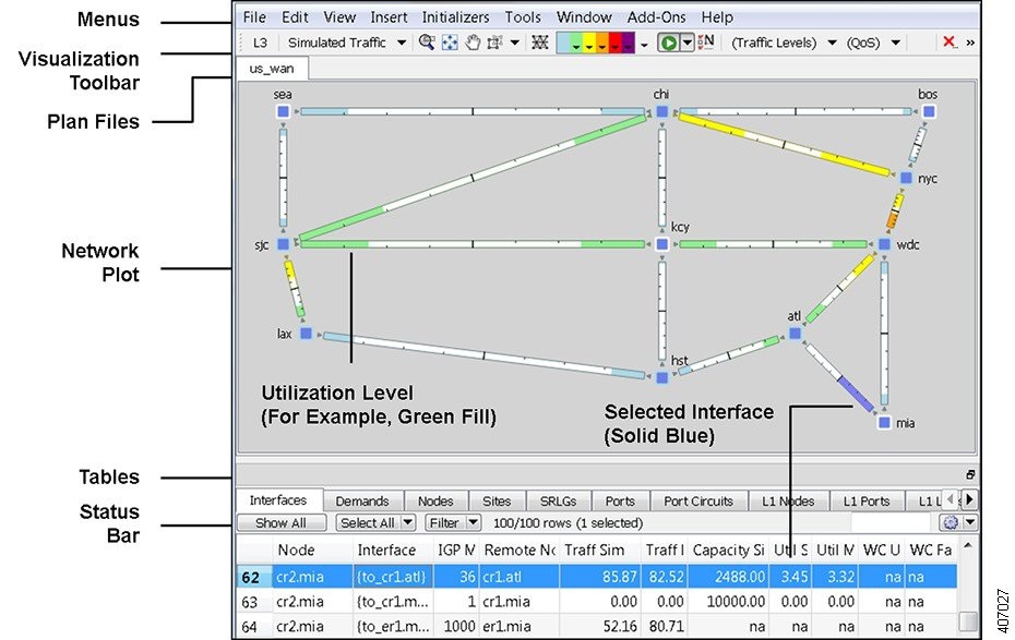
The WAE Design GUI is divided into the following primary sections. Figure 3-1 shows the GUI with a sample us_wan.txt plan in the network plot area.
- Menus—Menu selections for network modeling, simulation, and optimization.
- Visualization toolbar—Drop-down lists and icons that control how the network is displayed. For more information, see the Visualization Toolbar section.
- Plan file tabs—Identify which plan is currently opened. There can be multiple plans open; the tab with a white background is the active plan. To bring a plan to the forefront and make it the active plan, click its associated tab.
- Network plot—Displays a visual representation of the network topology. The color on each interface represents the percentage of traffic utilization on that interface. Rows that are selected in the tables, such as demands or interfaces, are highlighted in the plot with additional graphical attributes. For more information, see the View Network Plots section.
- Tables—Display network properties, including both measured and simulated information, for the network plan. For a list of default tables and information on how to interact with tables within the GUI, see the Tables section.
- Status Bar—Identifies the network simulation mode.
- Context menus—Enable you to right-click anywhere to view a list of actions that you can take. For more information, see the View Related Information section.
Figure 3-1 WAE Design User Interface
Visualization Toolbar
The Visualization toolbar (Figure 3-2) provides a convenient way to change the visual aspects of the network plot.
Figure 3-2 Visualization Toolbar
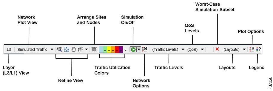
- Layout—A toggle button to change the view between Layer 3 (L3) and Layer 1 (L1). Note that you can also simultaneously view L3 and L1 networks. This is set in the Layer 1 tab of the Plot Options. For more information, see the Layer 1 Simulation chapter.
- Network Plot—A drop-down menu from which you choose the type of traffic displayed in the plot. For more information, see the View Network Plots section.
- Refine View icons—These icons enable you to refine and enhance your view in both in the network plot and in the site plots. For information, see the Refine Viewable Objects section.
- Arrange icon—Opens an Arrange palette that enables you to move selected nodes and sites into a selected schematic alignment.
- Utilization Color—Traffic utilizations are displayed by colors as a percent of available capacity used on that interface. This enhances the other visual cues, which is the length of the fill. You can change the colors and the utilizations they represent. For more information, see WAE Network Visualization Guide.

Note![]() All traffic is displayed in Mbps. In the network plot, the traffic utilization colors represent outbound traffic.
All traffic is displayed in Mbps. In the network plot, the traffic utilization colors represent outbound traffic.
- Simulation On/Off (white arrow in green circle) icon—By default, any change that voids the current simulation automatically triggers a resimulation. For instance, changes in topology trigger a resimulation. To turn off this resimulation, select the drop-down arrow next to the icon and deselect the “Auto resimulate” option. To turn it back on, reselect the this option.
- Network Options icon—Enables you to set global simulation modes, such as Full Convergence or Fast Reroute for MPLS, and whether to include multicast hops. You can also set IGP, BGP, and Multicast protocol options.
- Traffic Level—Drop-down menu of user-defined traffic levels in the plan. For more information, see the Traffic Demand Modeling chapter.
- QoS Level—Drop-down menu allowing the display of service classes, interface queues, and undifferentiated traffic. From the Manage QoS option, you can add/edit service classes, assign service classes to queues, and add/edit service policies. For more information, see the Quality of Service Simulation chapter.
- Worst-Case Simulation Subset (red X) icon—After a simulation analysis is performed over a specified set of failure scenarios (for example, circuits, nodes, and ports), you can click this icon to select which subset of these failure scenarios (for instance, circuits only), as well as service classes you want included in the worst-case analysis. This avoids having to run a second simulation analysis.
- Layouts—Drop-down menu of user-defined plots. For example, you might have schematic layouts, geographic layouts, street map layouts, separate layouts for different continents, simplified layouts with hidden nodes or sites, or other representations of the network. For more information, see the WAE Network Visualization Guide.
- Plot Options icon—Enables you to customize circuit width, text on interfaces, layouts (such as background images and geographic views), and other plot options. For more information, see the WAE Network Visualization Guide.
- Legend (question mark) icon—Displays a legend of icons and line types in the plot and their meanings. For more information, see the Plot Legend for Design Layouts chapter.
View Plots
WAE Design opens to the main network plot. Although WAE Design shows only the sites in the network plot and tables, you can view those sites in more depth. You can also view more depth of interfaces and demands in their respective plots. In addition to these plot views, you can create and view layouts that show only those portions of the network plot that you choose. For more information, see the WAE Network Visualization Guide.
View Network Plots
The network plot, also referred to simply as the plot, is the main area showing the network topology. It can contain both sites and nodes.
There are multiple network plot views available (top left of Figure 3-2). The default view is Simulated Traffic. To change the view, select it from the Network Plot View drop-down list in the far, left Visualization toolbar.
- Simulated Traffic—View of simulated traffic that can be used for capacity planning, what-if analysis, and failure planning. Circuits are sized proportional to their capacity. Interfaces are colored according to the percentage of simulated traffic (in comparison to available capacity as defined by the size of the interface or the QoS bound).
- Measured Traffic—View of traffic as measured from live views of the network. Circuits are sized proportional to their capacity. Interfaces are colored according to the percentage of measured traffic (in comparison to available capacity as defined by the size of the interface or the QoS bound).
- Worst-Case Traffic—Interfaces are colored to show the maximum utilization of the interface over all failure scenarios as defined by the most recently run simulation analysis. For more information, see the Simulation Analysis chapter.
- Failure Impact—Interfaces and nodes are colored to indicate how a failure of that interface or node would impact other interfaces and nodes. For more information, see the Simulation Analysis chapter.
- LSP Reservation—Circuits are sized proportional to their LSP reservable bandwidth. Interfaces are colored according to the percentage of bandwidth (in comparison to what is reserved for the LSP). For information, see the RSVP-TE Simulation chapter.
- By editing the plan file directly, you can add a user-defined static view to display interfaces with customized color fills and fill percentages. The view then appears as an option in the Network Plot drop-down list. For information, see the WAE Design Integration and Development Guide.
Although WAE Design focuses on IP/MPLS Layer 3 (L3) network views and traffic, you can also create and view Layer 1 topologies. To toggle between views of these two layers, use the View->Layer 1 View or View->Layer 3 View menus, or use the shortcuts Ctrl-1 for Layer 1 and Ctrl-3 for Layer 3. For information, see the Layer 1 Simulation chapter.
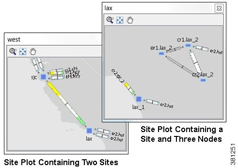
View Site Plots
The site plot can contain other sites and/or it can contain nodes and their connecting interfaces, including external interfaces that are labeled with their destination node (Figure 3-3).
To open a site plot, follow one of these steps.
- Double-click a single site from the plot.
- Select multiple sites from the plot and then double-click one of those sites.
- Select one or more sites from the plot or the Sites table.
–![]() Select View->Selected Sites.
Select View->Selected Sites.
–![]() Right-click and select Open Site View from the context menu.
Right-click and select Open Site View from the context menu.
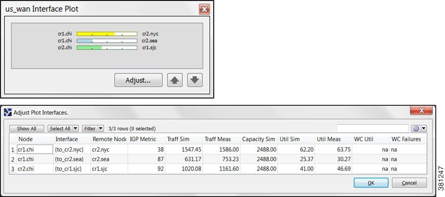
View Interface Plots
The interface plot is a window that displays selected interfaces in a stacked format, making it easier to compare one with another (Figure 3-4).
Step 1![]() Select one or more interfaces from either the Interfaces table or the plot.
Select one or more interfaces from either the Interfaces table or the plot.
Step 2![]() Open the interface plot in one of two ways.
Open the interface plot in one of two ways.
Following are further options for interface plots.
- To vertically move the interface list within the plot, click the up and down arrows.
- To view a table of the selected interfaces, click the Adjust button. A new Interfaces table appears.
- To sort the interfaces by ascending or descending order, follow these steps. The interface plot displays the interfaces according to the sort.
Click a column heading to toggle its sorting between ascending or descending order. Click OK.
Objects
Other than a site, an object is a representation of elements found in live networks, such as nodes (which represent routers), circuits, interfaces, LSPs, and more. A site is also an object, and is a WAE Design construct for simplifying the visualization of a network by grouping nodes within a site, or even by grouping sites within a site.
Objects have properties that identify and define them, many of which are discovered, though they can also be manually added and changed. For example, all circuits have a discovered Capacity property that can be edited. Other properties are derived. For example, Capacity Sim is derived from the Capacity property. Another example is that interfaces have a Util Sim property that identifies the percentage of Capacity Sim the simulated traffic is using. Properties are viewable and editable through an object’s Properties dialog box (right-click the object and select Properties). They are also viewable as table columns.
For more detailed information on object creating and editing, see the Plan Objects chapter.
Object Selections
Objects are selectable through tables and plots. However, not all objects are selectable from both, though most are. Some object types are only selectable through their tables, such as LSPs.
All selections made in a plot appear in the associated table and vice versa ( Table 3-1 ). Likewise, changes made in the plot are reflected in the tables, and vice versa. Hidden objects are excluded from the selection.
Table 3-1 assumes that all objects are in the foreground. For information on selecting objects that are in the foreground versus background, see the Refine Viewable Objects section.
Filter to Selected Objects
To filter only to the selected objects, select one or more objects from any plot or table, then select Filter->Filter to Selection. Alternatively, you can press and hold Ctrl-Shift (Cmd-Shift on Mac), and then double-click.
As with other object selections, to include the nested objects for site selections, add Alt to the selection process. For example, press and hold Alt while selecting one or more sites, and then select Filter->Filter to Selection.
Filter to Nested or Parent Objects
If a site contains multiple levels of child sites, you can filter to those nested objects. Right-click a site, and select Filter to Contained <Object> and then select one of the following, where <Object> equals sites, nodes, or L1 nodes.
- Direct—To see only the objects immediately contained within the site.
- All—To see all contained objects, no matter how deeply nested they are within child sites.
If a site contains only one level, the context menu changes to reflect as such.
Conversely, you can find a parent site for any given node. Select it, and then select Filter to Sites.
Refine Viewable Objects
View icons are available both in the network plot and in the site plots. Each of these icons make it easier to find what you need.
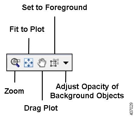
Except for Set to Foreground, when accessed through the Visualization toolbar, the view changes are applicable only to the network plot. When accessed through a site plot, the Zoom, Fit-to-Plot, and Drag actions apply only to that site plot.
Both the Zoom and Set to Foreground icons enable you to better focus and work in specific plot areas.
Shortcut = Press the letter “z,” which toggles this functionality on and off.
To escape from the Zoomed view, press Esc.
Shortcut = Press the letter “f,” which toggles this functionality on and off.
- Drag Plot—Enables you to move the cursor over any portion of the plot to drag it to a different location.
Shortcut = Press the letter “d” or press the icon again to toggle this functionality on and off. The feature remains enabled until you turn it off.
To escape from the Drag option, either press Esc or click the icon to toggle it off.
- Set to Foreground—Brings selected objects to the foreground for improved viewing while sending all other objects to the background where they appear as if they are transparent. Selected objects must be L3 nodes, L3 circuits, sites, L1 nodes, or L1 links. This feature does not apply to other objects, such as demands, LSPs, L1 circuits, and L1 circuit paths.
To escape the Set to Foreground option, click the icon to toggle it off while objects are selected.
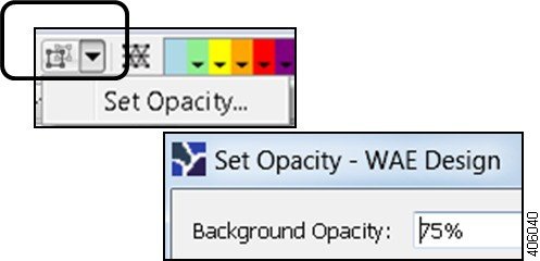
To increase or decrease the transparency (opacity) of how well the background objects appear, select the drop-down arrow next to the Set to Foreground icon. Enter the desired value, and click OK. The higher the value, the denser (darker) the background objects appear.
Note![]() If you are viewing both L3 and L1 objects, this opacity value for background objects takes precedence over the layout opacity value that is set for viewing different layers.
If you are viewing both L3 and L1 objects, this opacity value for background objects takes precedence over the layout opacity value that is set for viewing different layers.
Set Foreground and Background Preferences
To set foreground and background preferences, select the View->Preferences menu.
- Enable Selection of Background Objects—If this is enabled (selected), then you can select objects in the background. Otherwise, you cannot do so.
- Fit to Screen Zooms to Foreground Objects—If this is enabled (selected), then clicking the Fit-to-Plot icon zooms into and centers the selected objects. Otherwise, the plot itself is centered.
- Save Preferences—Save all view and tooltip preferences for all layouts when you save the plan file.
View Related Information
Tooltips
One method of seeing related information about an object is to show the tooltips and then hover the mouse over a site, node, L1 node, interface, or L1 link. For instance, hovering over a site you can see the number of contained L3 nodes, L1 nodes, and sites, as well as the total number of interfaces connected to the contained L3 nodes. To toggle this tooltip on or off, select the View->Preferences->Show Tooltips.
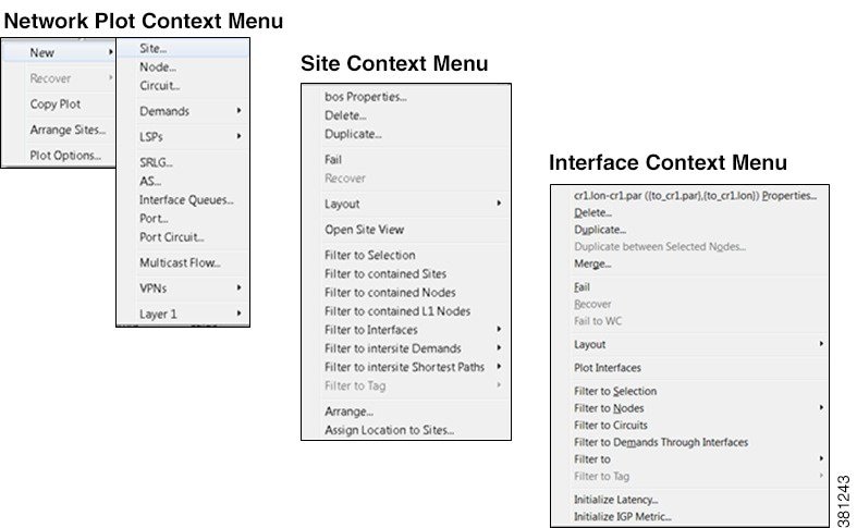
Context Menus
WAE Design has a hidden menu called a context menu (Figure 3-5). Anywhere that you right-click, whether it is in an empty area in the plot, on an object in the plot, on a table tab, or on a column or row in a table, a context menu appears giving you available options based on where you clicked. The only areas this context menu does not apply is in the main menus and in the Visualization toolbar.
The most common use case for context menus is for filtering to related objects. For example, to find the L1 circuits mapped to an L3 circuit, right-click the L3 circuit and select Filter to L1 Circuits from the context menu. You can select multiple objects and right-click just one to find the related information for all selected objects. If needing to see only selected objects in a table, right-click one of the selected objects and select Filter to Selections.
To access a context menu, right-click any empty area of a plot or right-click one or more objects from the network plot or table. If in a site, an interface, or a demand plot, the actions taken affect the network plot.
Figure 3-5 Examples of Context Menus
Tables
The tables that are viewable from the WAE Design GUI display a series of rows and columns, wherein the rows are objects and the columns are properties (Figure 3-6). Plan files also contain other tables that are not viewable from the GUI. These tables contain more complex information, such as showing complex relationships between objects. If you open a plan file using a.txt editor, each table is labeled with angle brackets, such as <Nodes> and <Sites>.
Note![]() For detailed information about plan files and tables, as well as information on creating user-defined columns and tables, see the WAE Design Integration and Development Guide.
For detailed information about plan files and tables, as well as information on creating user-defined columns and tables, see the WAE Design Integration and Development Guide.
Common Tables
There are numerous tables available for specialized purposes, such as Multicast, P2MP LSPs, and Ports default. The tables listed below are the most commonly used and are the defaults. For information on showing and hiding tables, see Show or Hide Tables or Columns.
To bring a table to the forefront and make it the active table, click its associated tab. For example, to open the LSP table, click the LSP tab.
- Interfaces—A list of the interfaces in the network.
- Demands—A list of the demands in the network. Each demand specifies how much traffic is routed from a source (node, external AS, or external endpoint) to a destination (node, external AS, external endpoint, or multicast flow destination).
- Shortest Path—A list of the routes between selected sites.
- Nodes—A list of network routers, which typically have names that suggest their location and function. For example, node cr1.atl is core router 1 in the Atlanta site.
- LSPs—A list of MPLS LSPs in the network; each LSP contains both a source and destination. Note that sub-LSPs within point to multipoint (P2MP) LSPs are listed in the LSP table.
- Sites—A list of network sites.
- SRLGs—A list of the shared risk link groups (SRLGs); an SRLG is a group of objects that might all fail due to a common cause.
- AS—A list of both internal and external autonomous systems (AS’s). An AS is a collection of connected IP routing prefixes that are controlled by one operator.
Figure 3-6 Common Table Functions
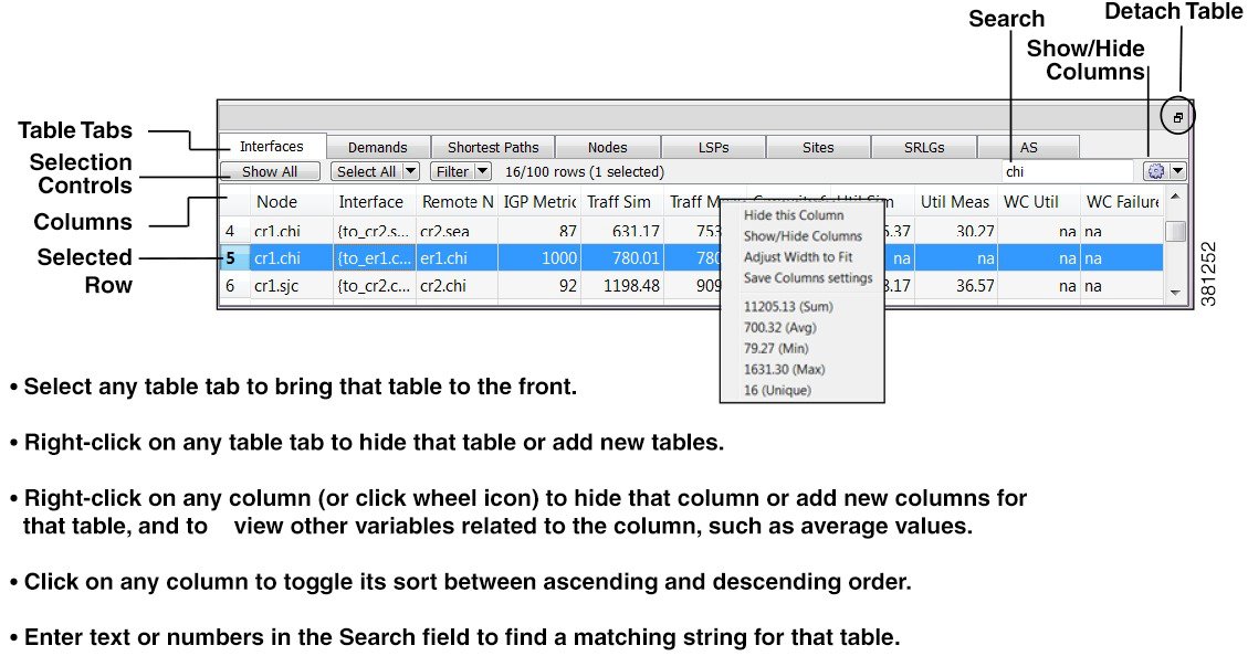
Show or Hide Tables or Columns
Search and Filter in Tables
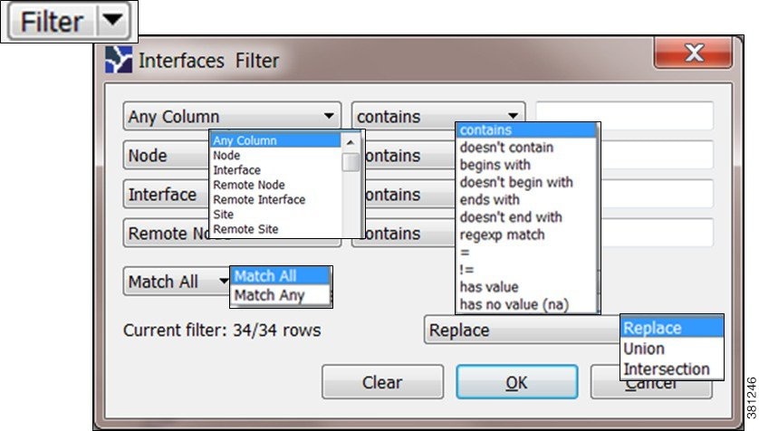
Most WAE Design tables, whether below the network plot or with dialog boxes, have an empty Search field in the top right as shown in Figure 3-6. Likewise, they usually have a Filter control menu that opens a Filter dialog box specific to that table. Figure 3-7 is an example of an Interfaces Filter dialog box.
|
|
|
|---|---|
1. 2. |
|
Filter the table to a list of specific search values, and either replace, add to, or narrow the list of objects currently showing in a table. |
1. 2. 3. 4. – – 5. – – – |
Filter the selection to associated objects. For example, you might want to filter a circuit to associated interfaces. |
Select the Filter -> Filter to X control menu, where X is a name of a viable object. |
Toggle whether to change the filter selection with or without first asking. |
Select the Filter -> Interaction with current filter -> X, where X is either Always Ask or Replace. |
Save Table Settings or Return to Defaults
Other Table Actions
Log and Report Windows
The following additional windows are displayed using menu items or after running tools.
- Log window—This window appears automatically when warnings or errors are logged. You can view these by selecting the Window->Log Window menu.
- Reports—Reports are generated through the Tools->Reports menu, as well as automatically when running certain tools such as Simulation Analysis. The report window appears at that time, and is accessible later by selecting the Window->Reports menu. For more information, see the Reports chapter.
Related Topics
- Plan Objects chapter
- Plot Legend for Design Layouts chapter
- WAE Network Visualization Guide
- WAE Design Integration and Development Guide
 Feedback