A Day in the Life of a Prompt White Paper
Available Languages
Bias-Free Language
The documentation set for this product strives to use bias-free language. For the purposes of this documentation set, bias-free is defined as language that does not imply discrimination based on age, disability, gender, racial identity, ethnic identity, sexual orientation, socioeconomic status, and intersectionality. Exceptions may be present in the documentation due to language that is hardcoded in the user interfaces of the product software, language used based on RFP documentation, or language that is used by a referenced third-party product. Learn more about how Cisco is using Inclusive Language.
The rise of Large Language Models (LLMs) has introduced a new paradigm of interaction: the “prompt.” While widely used across industries, the underlying mechanics of how a prompt is processed—from user input to generated response—remain largely opaque. This document demystifies that journey in detail, following a prompt as it traverses networks, control planes, compute systems, and GPU fabrics.
At a high level, LLM inference is not a single operation, but a multi-stage distributed pipeline involving:
● Network transport, carrying requests across the internet and within data centers
● Control plane systems, such as API gateways and LLM routers, making policy and routing decisions
● CPU-based processing, performing parsing, tokenization, and scheduling
● GPU-based execution, handling the computationally intensive inference tasks
● High-performance interconnects, enabling coordination across multiple GPUs
● Streaming mechanisms, delivering responses incrementally to users
This architecture closely mirrors modern distributed networking systems. A prompt behaves like a flow: it is routed, queued, processed, and streamed back, often traversing multiple domains with different latency and performance characteristics.
A key concept explored in this document is the existence of two distinct but interconnected fabrics:
● The request network (north-south), based on IP protocols (TCP/TLS), which carries prompts to inference systems
● The GPU fabric (east-west), based on NVLink, InfiniBand, or Remote Direct Memory Access (RDMA) over Ethernet, which enables distributed model execution
Understanding the boundary between these two domains is essential for analyzing performance, scalability, and reliability.
From a latency perspective, current inference systems are largely dominated by compute factors—particularly batching delays and prompt processing (prefill). As a result, network latency has historically been a secondary concern. However, this may be about to change.
As inference hardware evolves and inter-token latency decreases, and as agentic AI workflows introduce significantly more “chattiness” (multiple sequential LLM calls per user request), the relative contribution of network latency becomes increasingly significant. In emerging scenarios, network delays can account for a meaningful portion of total response time.
This leads to a critical conclusion:
AI inference is becoming a networking problem again.
This shift has profound implications:
● Inference workloads will need to move closer to users, reducing round-trip latency
● Distributed inference architectures will become the norm, spanning edge, metro, and core locations
● Network performance, topology, and placement will directly impact AI application experience
● Service providers have a unique opportunity to play a central role in the AI inference value chain
For network engineers and architects, this represents a familiar challenge in a new domain. The same principles used to design high-performance, low-latency networks—traffic engineering, locality, distributed systems design—are becoming directly applicable to AI infrastructure.
In short, understanding the lifecycle of a prompt is no longer just an academic exercise. It is foundational to designing the next generation of AI-enabled systems and services.
The term “prompt” has become already part of our life, whether we work in an engineering field, or legal, or HR, or marketing. Everyone knows what a prompt is, but very few people know what the day in the life of a prompt looks like. And you don't have to know, but if you are in networking, you should understand well, because it matters. The goal of this paper is to go through the complicated life of a prompt from the moment you type it in your AI Assistant until you get a response. The paper explores this in a level of detail so anyone in our networking field can understand what all is happening, even if you are not a GPU expert.
The following diagram captures the key elements on the complicated prompt’s life we will explore in the document:
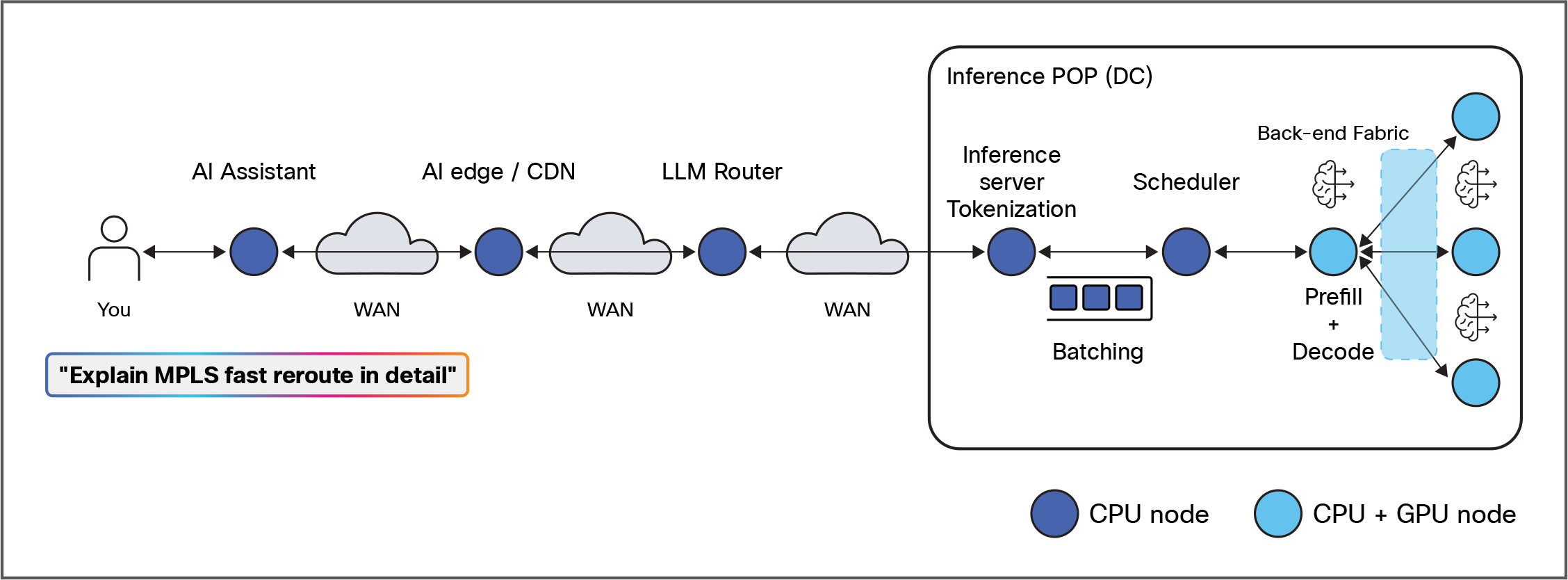
End-to-end AI Inference process
From keystroke to GPU and back again
Let's start with a simple assumption: A user types a prompt into a web UI (ChatGPT-like interface, enterprise assistant, or embedded copilot). What happens next is a multi-stage distributed pipeline spanning client software, IP networks, API gateways, inference routers, tokenizers, GPU schedulers, and distributed model execution across multiple accelerators.
Client-side: Prompt creation and submission
The journey begins in a browser or application:
● The user types: “Explain MPLS fast reroute in detail”
● The UI may:
◦ Add system prompts (hidden instructions)
◦ Attach conversation history
◦ Apply formatting or safety metadata
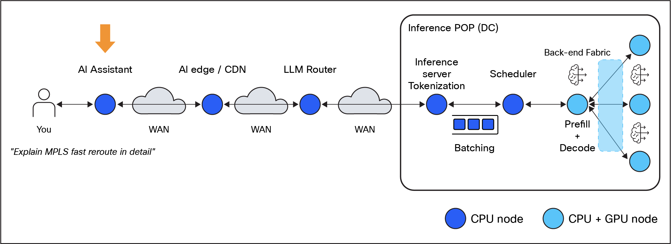
User request captured as the input prompt
At this stage, the request is assembled into a structured payload, typically JavaScript Object Notation (JSON):
| POST /v1/chat/completions Authorization: Bearer <token> { "model": "llama-3-70b", "messages": [ {"role": "system", "content": "You are a network expert"}, {"role": "user", "content": "Explain MPLS Fast reroute in detail..."} ], "temperature": 0.2, "stream": true |
The First Hop: Internet Transport
The request leaves the client:
● DNS resolution → resolves API endpoint
● Transmission Control Protocol (TCP) 3-way handshake (or Quick UDP Internet Connections [QUIC] if HTTP/3)
● Transport Layer Security (TLS) handshake (cert validation, key exchange)
Then:
● HTTPS POST request is transmitted over IP
● Routed through:
◦ ISP edge
◦ Internet backbone
◦ Possibly Content Delivery Network (CDN) edge
The request is sent via:
● HTTPS over TLS 1.2/1.3
● HTTP/2 or HTTP/3 (QUIC increasingly common)
Key components:
● DNS resolution (possibly via GeoDNS or Anycast)
● TLS termination may occur later at edge or gateway
Edge network and API gateway layer
After the request leaves the user network, it typically hits:
● CDN / Edge: Cloudflare, Akamai
● API Gateway: Kong, Apigee, Amazon Web Services (AWS) API Gateway
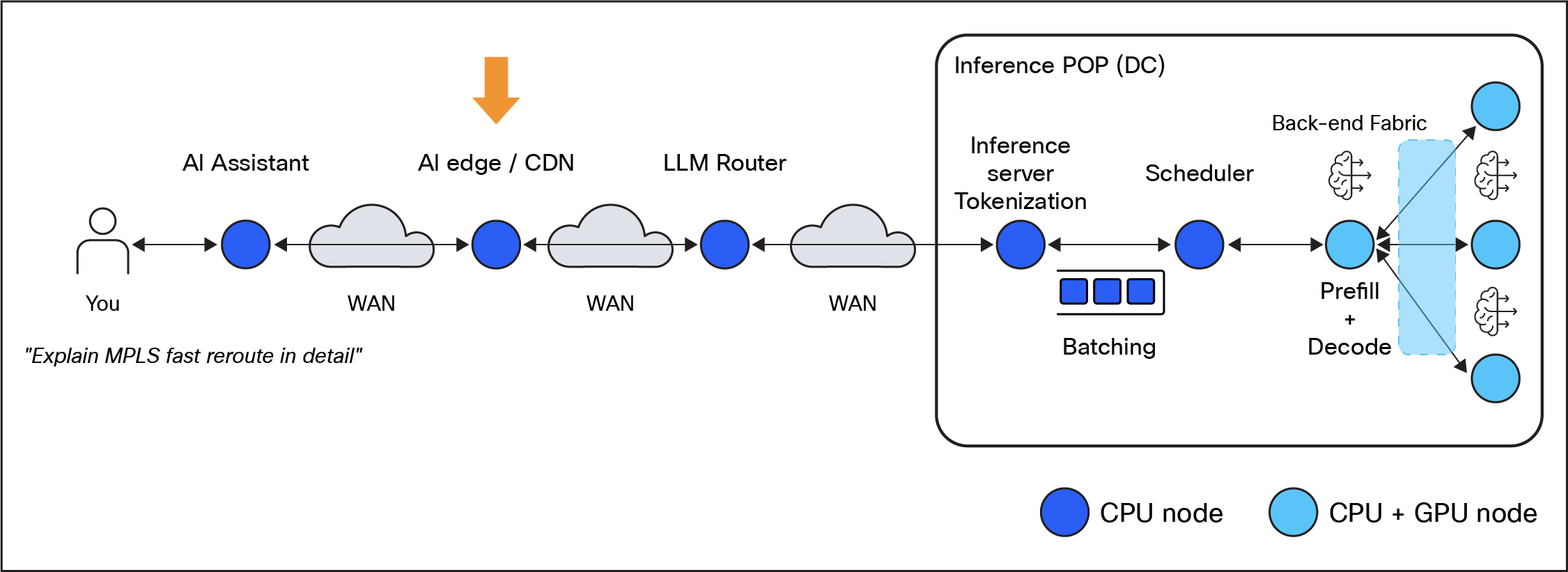
Edge processing
API gateway / Edge layer
Common elements here:
● Kong Gateway
● Apigee (Google Cloud API Management)
● AWS API Gateway
● NGINX / NGINX Plus
● Envoy Proxy
Responsibilities:
1. Authentication
◦ API keys / OAuth tokens / JSON Web Token (JWT) validation
◦ Rate limiting per user / tenant
2. Policy enforcement
◦ Prompt length limits
◦ Tenant-level routing rules
◦ Data residency constraints
3. Logging and observability
◦ Request tracing (OpenTelemetry spans)
◦ Audit logs (critical for enterprise LLM usage)
4. Request routing decision
◦ Which LLM?
◦ Which region?
◦ Which inference cluster?
At this stage, the processing is done by systems like:
● LiteLLM proxy
● OpenRouter
● Azure AI Gateway
● AWS Bedrock routing layer
Which may act as “model routers,” abstracting multiple backend LLM providers.
LLM Router / Model Gateway layer
This is a critical emerging control plane component. It may appear after the CDN edge or before, depending on who is managing or controlling the LLM Router function.
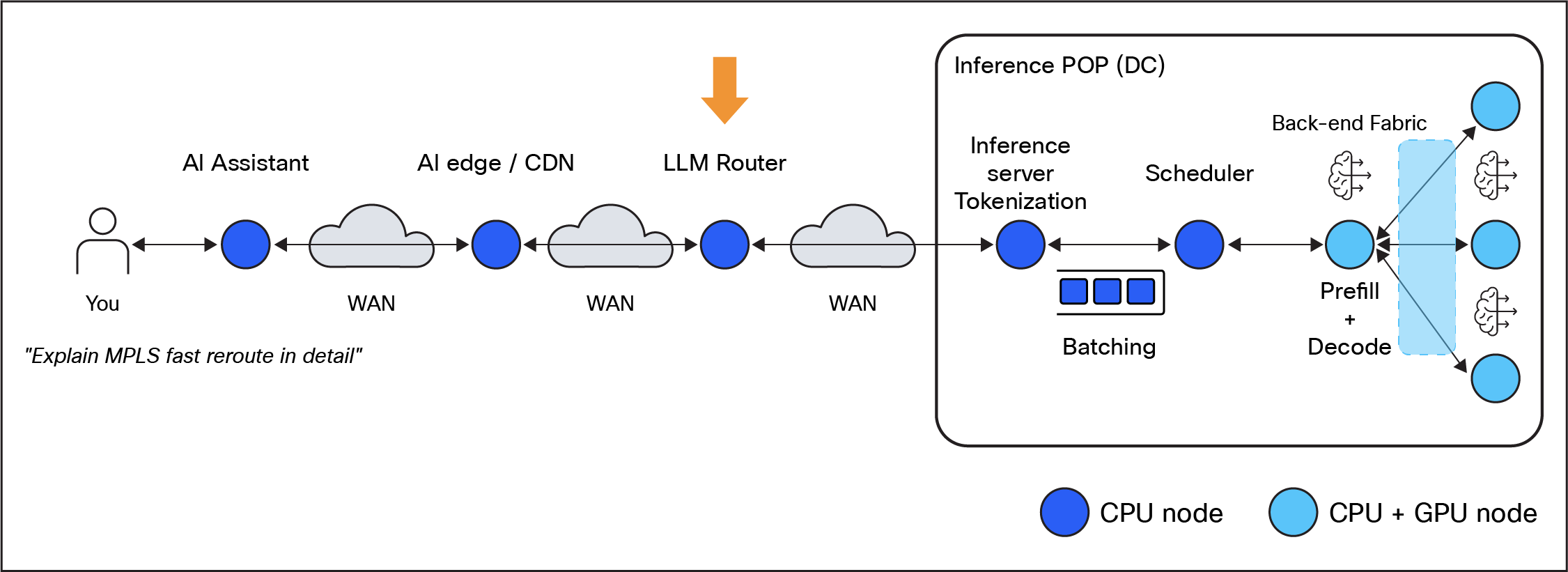
Intelligent Inference optimization at the LLM Router
Examples:
● LiteLLM (open-source)
● OpenRouter (commercial aggregation layer)
● LangDB
● Portkey
● Azure AI Model Router
● AWS Bedrock inference routing
● Databricks Model Serving router
Responsibilities:
● Select model (GPT-4, Claude, Llama, etc.)
● Apply fallback policies (failover between models or providers)
● Enforce cost / latency trade-offs
● Potentially rewrite prompts (prompt engineering layer)
● Load balancing across inference clusters
● Policy enforcement (data sovereignty, filtering)
This is where policy meets inference economics.
Inference API front-end (serving layer)
Once routed through the WAN network, the request enters the inference infrastructure (some form of Data Center where inference will happen).
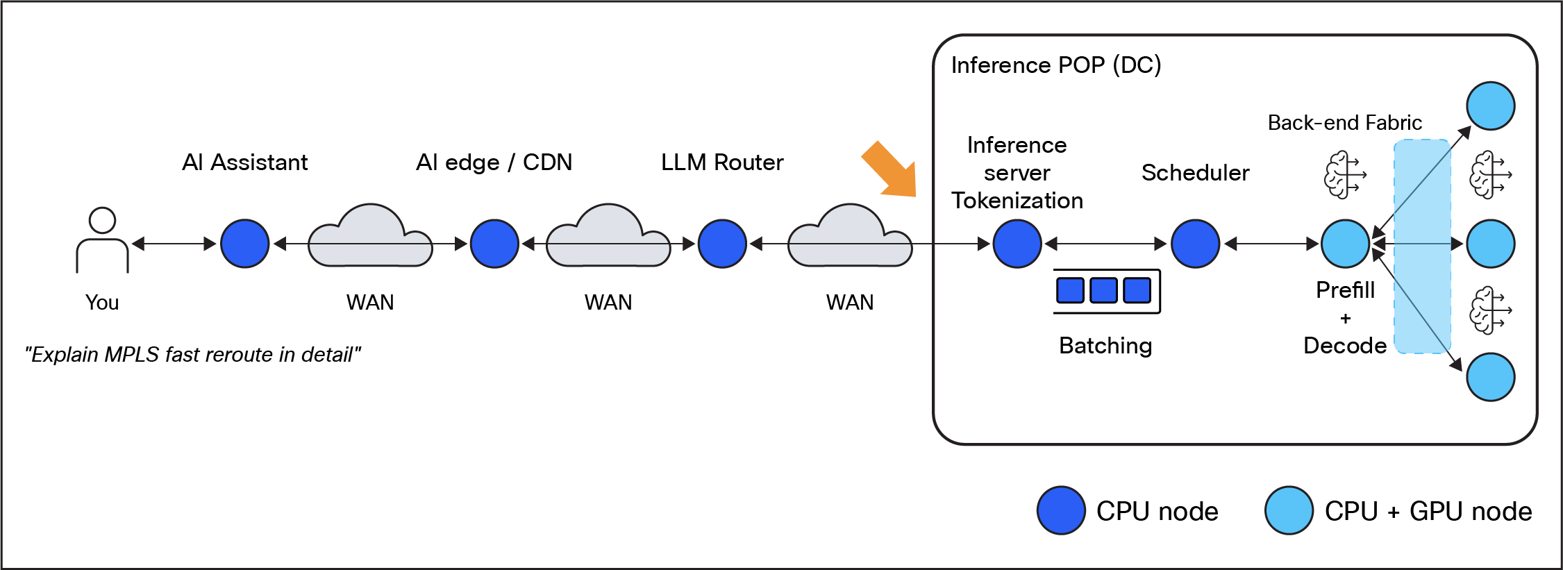
The prompt reaches the Inference Data Center
Typical serving stack:
● vLLM (very common in modern deployments)
● TGI (Text Generation Inference by HuggingFace)
● TensorRT-LLM / NIM (NVIDIA)
● DeepSpeed-Inference (Microsoft)
● Ray Serve (for orchestration)
● SGLang / LMDeploy (increasingly used)
Multiple steps happen here, let's break it down. This is where the “WAN network” ends and where the “GPU fabric begins.”
First contact: NIC → CPU (ingress into the inference cluster)
When the request arrives at the inference cluster node, it always lands on a network interface card (NIC):
● Packet is processed by:
◦ Kernel network stack (Linux TCP/IP)
◦ Or accelerated path (Data Plane Development Kit [DPDK], Extended Berkeley Packet Filter [eBPF], eXpress Data Path [XDP] in high-performance setups)
At this point:
Everything is still CPU-bound and network-bound.
API / inference server process (CPU domain)
Now the request is inside a user-space process, typically:
● vLLM server
● Text Generation Inference
● TensorRT-LLM backend
What happens here:
Request parsing
● JSON deserialization
● Headers inspection
● Authentication (if not already done upstream)
Tokenization (CPU-heavy stage)
● Uses:
◦ HuggingFace tokenizer
◦ SentencePiece
◦ tiktoken
Important characteristics of the processing at this stage:
● This is pure CPU work
● Often parallelized across threads
Tokenization stage (CPU side)
Before GPUs do anything, the prompt is tokenized.
Tools used:
● HuggingFace Tokenizers (Rust-backed fast tokenizer)
● SentencePiece (Google)
● OpenAI tiktoken
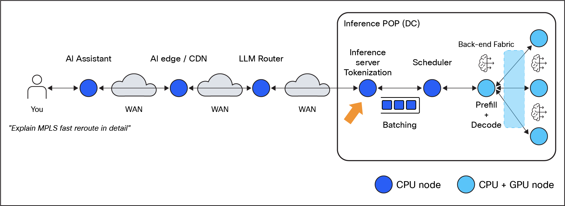
Prompt Tokenization
Example transformation:
Input:
“Explain MPLS fast reroute”
Becomes tokens:
| [4512, 99821, 3921, 1204, ...] |
Important detail:
● Tokenization is CPU-bound
● Often vectorized and parallelized per request batch
● Token vocab size: 30k–200k tokens depending on model
The scheduler: where decisions are made
Now comes the critical piece: the scheduler.
This is not a single “thread”—it’s a coordinated system inside the inference server.
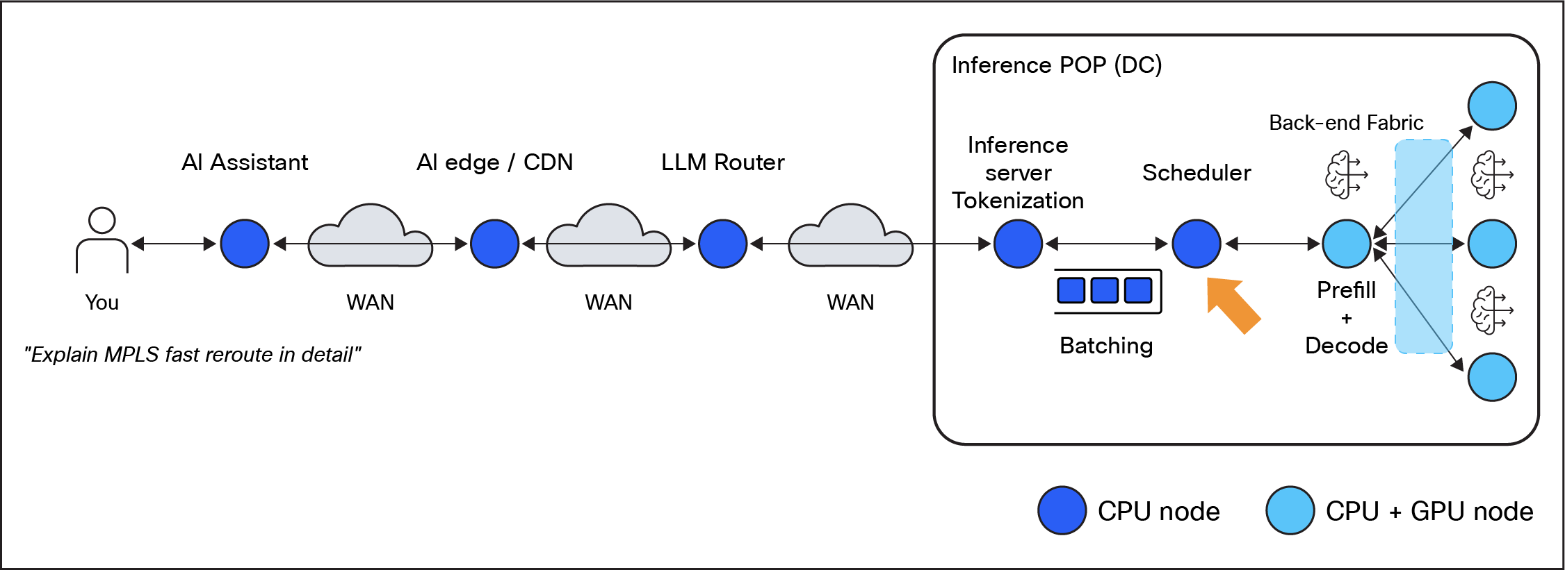
Request batching and scheduling
Typically, requests are not served “one-by-one.” Efficiency of the hardware (GPU) utilization would be extremely low and the cost-per-token too high. Therefore, requests are usually batched, so there is a trade-off between latency (requests must wait until the batch is full) and efficiency/cost (hardware is highly utilized if several requests are processed in a batch in parallel).
Responsibilities:
● Maintain request queues
● Perform dynamic batching
● Decide:
1. Which GPU?
2. Which node?
3. When to execute?
Local vs remote scheduling decision
At this point, the system may:
Case A: Execute locally
● If GPU capacity is available
● If model is resident on this node
→ No additional network hop required
Case B: Forward to another node (important)
In case:
● GPUs are saturated
● Model not present locally
● Load balancing policy requires it
Then:
The request is forwarded over the data center network to another server
This is a second network hop.
In many architectures, routing decisions are ideally made before tokenization to avoid additional latency. However, some systems may still forward requests post-tokenization when performing fine-grained load balancing or model-specific scheduling.
Inter-node hop (CPU network again)
This looks like:
● gRPC / HTTP call between inference nodes
● Happens over:
◦ Ethernet (typical DC fabric)
◦ Or service mesh (Envoy sidecars)
Path:
| Node A (CPU) → NIC → DC switch fabric → NIC→Node B (CPU) |
Important:
● Still no GPU involved yet
● This is standard IP networking
Arrival at execution node (GPU-serving node)
Now the request reaches the node that will actually run inference.
Same ingress path again:
● NIC → kernel → user-space
Then:
Tokenization may or may not be repeated
● Some systems forward already tokenized input
● Others re-tokenize (less efficient but simpler)
Prefill phase (GPU execution begins)
Now we enter GPU computation. Now the request enters the GPU execution queue.
● Request placed into:
◦ Prefill queue
◦ Decode queue (later)
● Scheduler forms a batch:
◦ Groups multiple requests
◦ Aligns sequence lengths
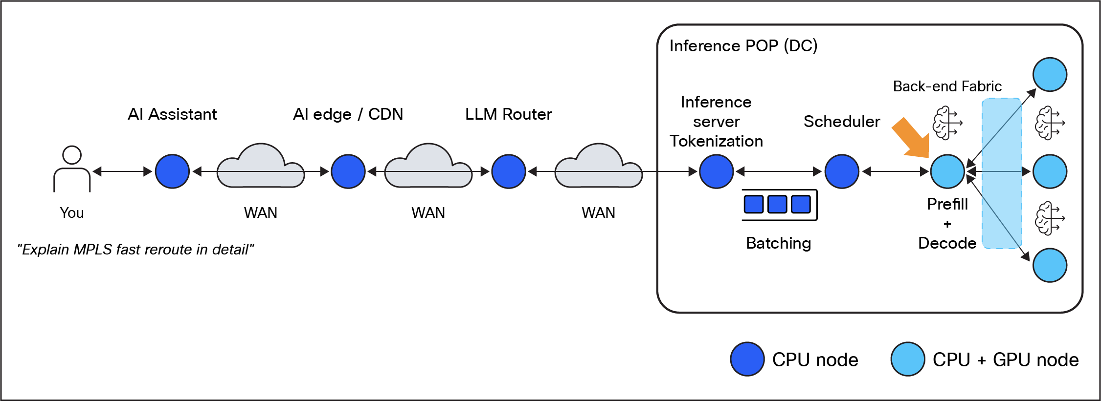
GPU domain: Prefill and decode
Critical transition
This is the moment where we move from network/CPU domain → GPU domain
CPU → GPU data transfer
Before execution:
● Token IDs must be copied to GPU memory
Mechanism:
● PCIe transfer (or NVLink if CPU-GPU unified memory system)
● DMA (Direct Memory Access)
Path:
| CPU RAM → PCIe → GPU High Bandwidth Memory (HBM) |
Latency:
● Small but non-negligible (~10–50 microseconds)
The model inference has two phases:
Prefill (a.k.a. prompt processing)
This stage:
● Processes the entire input prompt
● Builds the KV cache (Key-Value attention cache). This is state that is necessary for the Transformer model to do inference. The KV cache is built during prefill and then incrementally extended during decoding, allowing the model to reuse prior context without recomputing it.
GPU behavior:
● General Matrix-Matrix Multiplications (GEMMs)
● Attention over full context window
● Memory bandwidth bound (not compute bound in many cases)
Software stack:
● Compute Unified Device Architecture (CUDA) kernels
● cuBLAS / cuDNN
● FlashAttention (critical optimization)
● TensorRT kernels (if NVIDIA stack)
Model parallelism (when the model is too large for one GPU)
This is where multi-GPU systems come in.
Types of parallelism for Inference
Tensor Parallelism
Model layers are split across GPUs.
Example:
● Layer weights split column-wise
● Each GPU computes part of the matrix multiplication
Used by:
● TensorRT-LLM
● DeepSpeed
● Megatron-LM
Pipeline Parallelism
Different layers on different GPUs:
| GPU0: layers 1–10 GPU1: layers 11–20 GPU2: layers 21–30 |
Activations flow GPU-to-GPU.
Expert Parallelism (Mixture of Expert [MoE] models)
Used in:
● Mixtral
● DeepSeek MoE variants
Only subsets of model ("experts") are activated per token.
Multi-GPU execution (if required)
If model does not fit in one GPU:
Intra-node (NVLink)
| GPU0 ↔ GPU1 ↔ GPU2 ↔ GPU3 |
● Tensor slices exchanged
● Attention results aggregated
Transport:
● NVLink / NVSwitch
● Ultra-low latency
Inter-node (InfiniBand / RoCE)
If model spans nodes:
| Node A GPU ↔ NIC (RDMA) ↔ InfiniBand or Ethernet ↔ NIC ↔ Node B GPU |
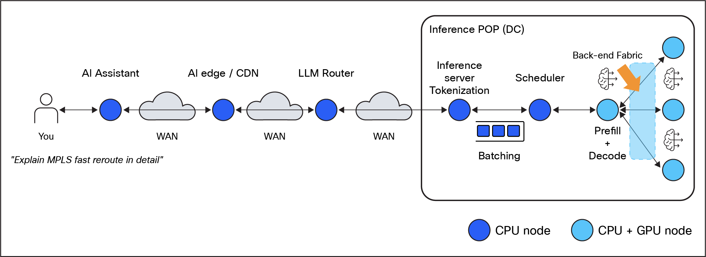
Back-end Fabric
Key technologies:
● RDMA (bypasses CPU) or RDMA over Ethernet (RoCE)
● NCCL for collectives
Important distinction:
This is NOT TCP/IP traffic in the classical sense.
It is:
● RDMA verbs
● Zero-copy memory transfers
At this point we have two completely different “networks”:
Request network (north-south)
● HTTP / TCP / TLS
● CPU handled
● Used before GPU execution
GPU fabric network (east-west)
● NVLink / InfiniBand / RoCE
● RDMA-based
● Used during inference
RoCE operates over Ethernet but uses RDMA semantics, bypassing the traditional TCP/IP processing path, effectively behaving more like a memory transport than a packet network.
Decode phase (token generation loop)
After prefill, the model enters an autoregressive loop:
| while not finished: predict next token sample token append to context |
This is the decode phase.
Key characteristics:
● One token at a time (sequential dependency)
● Highly latency-sensitive
● KV cache reused (critical optimization)
Now for each generated token:
● GPU computes next token
● If multi-GPU:
◦ Synchronization across GPUs
● Result stored in GPU memory
Optimizations used in production:
● Speculative decoding (e.g., smaller model proposes tokens)
● Continuous batching (vLLM innovation)
● KV cache paging (vLLM “PagedAttention”)
● Quantization (FP8, INT8, INT4)
Output streaming back to user
As tokens are generated:
● Sent incrementally over HTTP chunked responses
● Often via:
◦ Server-Sent Events (SSE)
◦ WebSockets
◦ HTTP/2 streaming
Example:
| Explain → MPLS → fast → reroute → is → ... |
Each token is:
● Immediately transmitted
● Rendered in UI
● Possibly post-processed (formatting, safety filters)
GPU → CPU → Network (reverse path)
Now we reverse direction:
GPU → CPU transfer
| GPU HBM → PCIe → CPU RAM |
● Token IDs copied back
CPU processing
● Token → text decoding
● Optional filtering
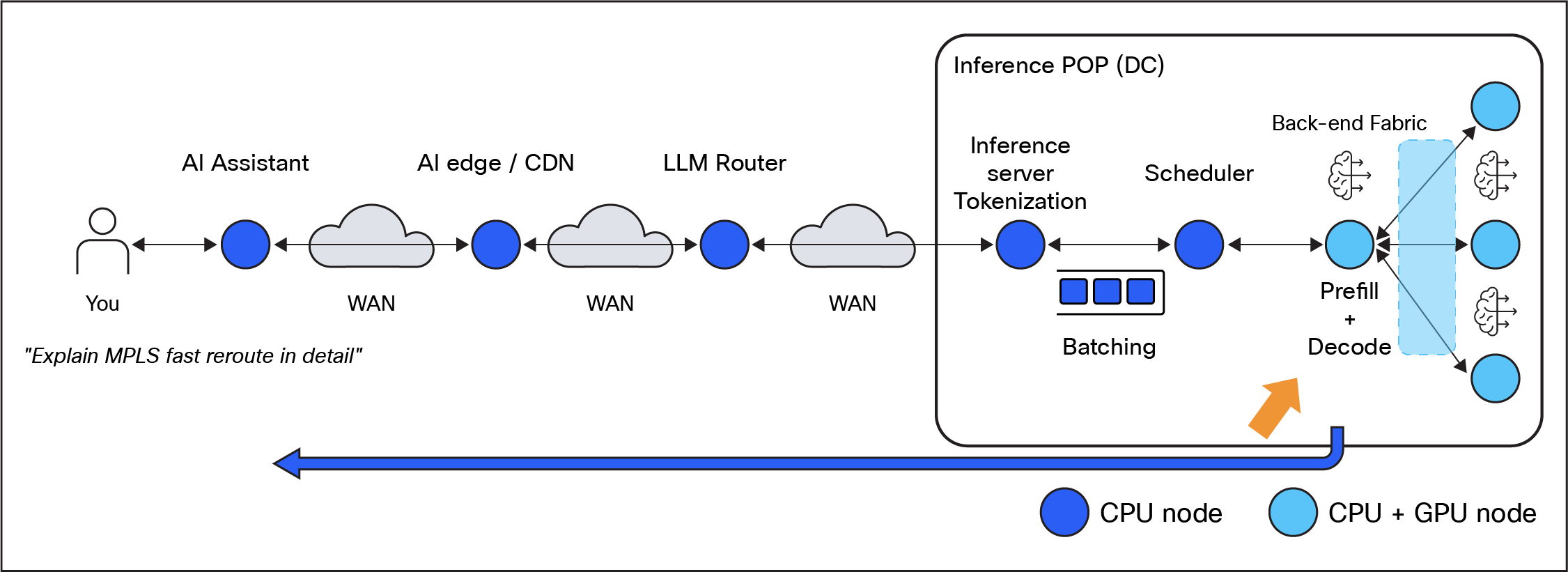
Decode generation and streaming back to user
Network transmission
| CPU → socket → NIC → network → client |
Streaming:
● SSE / WebSockets
● Token-by-token
Post-processing layer
Before final delivery there may be some possible additional steps, depending on the Inference provider:
Safety filtering
● OpenAI Moderation API
● NVIDIA NeMo Guardrails
● Azure Content Safety
● Anthropic Constitutional AI filters
Structured output enforcement
● JSON schema validation
● Tool calling (function calling frameworks)
Logging and telemetry
● Prometheus metrics
● OpenTelemetry traces
● Observability tools (Splunk)
Putting it all together (end-to-end timeline)
1. User types prompt in UI
2. HTTPS request sent via IP network
3. API Gateway authenticates + enforces policy
4. LLM router selects model + region
5. Request enters inference server (vLLM/TGI/TensorRT-LLM)
6. Tokenization happens on CPU
7. Prefill phase runs on GPU cluster
8. KV cache is constructed
9. Decode loop generates tokens sequentially
10. Tokens streamed back to user
11. Safety + logging + observability layers finalize request
For network engineers, the key insight is:
| LLM inference is not a single “AI operation” — it is a distributed systems + networking + GPU scheduling problem disguised as a chatbot. |
How long does this process take?
Total inference latency perceived by the user is a combination of several factors:
● Time to First Token (TTFT): Time it takes for the LLM to generate the first token after inference request happens. It includes the network latency.
● Inter-Token Latency (ITL): How fast the LLM inference system is able to generate the response tokens.
So, we can consider that the total perceived latency can be computed using this formula, assuming N is the number of tokens of the response:
T_response ≈ TTFT + (N-1)* ITL
Now, let's try to put some numbers and orders of magnitude on these variables, and explore later what is the relevance of network latency.
TTFT (Time to First Token) decomposition
TTFT is where most misunderstandings happen. It’s not “just compute.”
Let’s break it down rigorously:
TTFT ≈ T_queue + T_tokenize + T_prefill + T_network
Queueing delay (T_queue)
Dominant in many systems. Depends greatly on the load of the inference service.
Factors:
● Batch formation window (dynamic batching)
● Load level (RPS vs GPU capacity)
● Scheduling algorithm ((first-in, first-out [FIFO], priority, fairness)
Typical ranges:
● Light load: ~5–20 ms
● High load: 50–300+ ms
TTFT is often dominated by waiting, not computing.
Tokenization time (T_tokenize)
CPU-bound:
● HuggingFace tokenizer / tiktoken
● Vectorized string parsing
Typical:
● Small prompt: 1–5 ms
● Large prompt (3k tokens): 5–20 ms
Usually negligible unless poorly optimized.
Prefill compute (T_prefill)
This is the real GPU-heavy part.
Depends on:
● Prompt length (N tokens)
● Model size (parameters)
● Parallelism efficiency
Rough intuition:
| T_prefill ∝ O(N × model_layers × hidden_dim) |
Typical:
● Small prompt (1k tokens): 50–150 ms
● Large prompt (8k tokens): 200–800 ms
Network overhead (T_network)
Includes:
● Client → edge Round-Trip Time (RTT)
● Gateway → inference cluster
● Internal DC latency
Typical:
● Internet RTT: 20–80 ms
● DC internal: <1–5 ms
Usually negligible today, but let's discuss this more later how this may change.
Putting it together
Example realistic TTFT:
| Component |
Time |
| Queueing |
120 ms |
| Tokenization |
10 ms |
| Prefill |
180 ms |
| Network |
40 ms |
| Total TTFT |
~350 ms |
ITL depends on how fast the inference hardware (GPUs) can generate new tokens for a given request. As we have seen, the token generation is an iterative process that generates "one token at a time" by running a loop that finishes when the model produces an <EOM> (End of message) token or when the response reaches the maximum number of allowed tokens. During that process, the system is generating individual tokens (portions of the response) that can be streamed back to the user or accumulated to send the entire response at the end. Either way, the client will see only the complete response once all the tokens have been generated and forwarded.
Different hardware architectures and generations have different performance levels in terms of the tokens per second. Also, the ITL offered is dependent on the model size and characteristics. Here are some examples:
| Model type |
Model |
Inter-token latency |
| Slower but very strong capability-oriented models |
Claude Opus 4.6 |
23–25 ms/token |
| Fast strong proprietary/frontier APIs |
PreviewGrok 4 Fast Gemini 3.1 Pro Preview GPT-5.4 |
~6.7 ms/token ~8.7 ms/token ~11.9 ms/token |
| Fast strong reasoning/open deployments |
DeepSeek V3.1 Reasoning DeepSeek V3.1 Terminus |
~3.5 ms/token ~6.5 ms/token |
| Best current inference-service result for a genuinely strong open model |
Fast HW serving gpt-oss-120B (high) |
~0.47 ms/token |
| Best publicly cited extreme specialized result |
Inference HW vendor + Llama 3.1 8B |
~0.06 ms/token |
The following graph is from a recent test where a few hardware technologies were benchmarked for a given model of reference. We are not exposing the inference hardware vendor names because the focus here is only to show how inference speed is evolving over time as new generations of hardware are released.
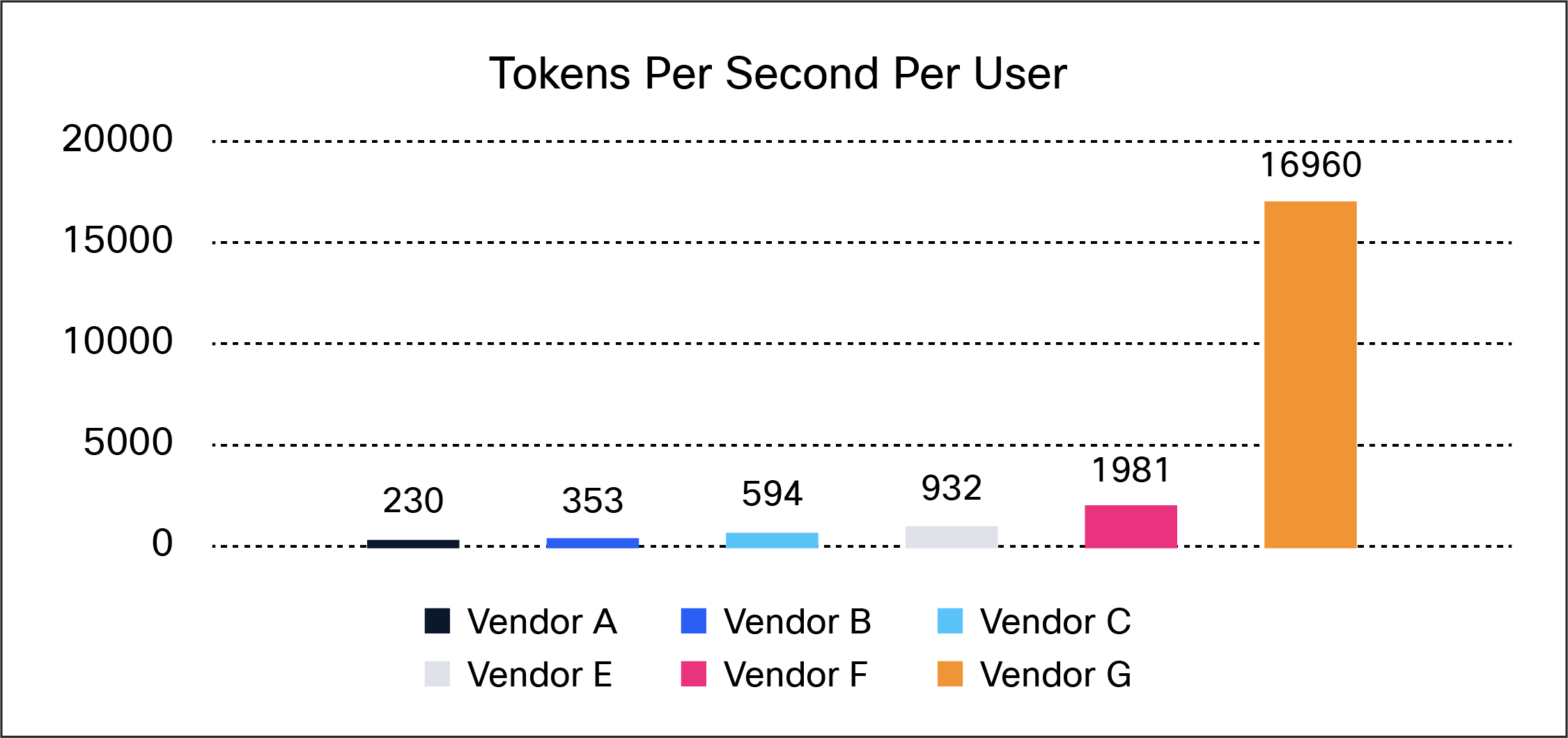
Evolution of Inference speed across different GPU/Hardware generations
We can, however, visualize the same data from a perspective of the per-user Inter-Token Latency perceived:
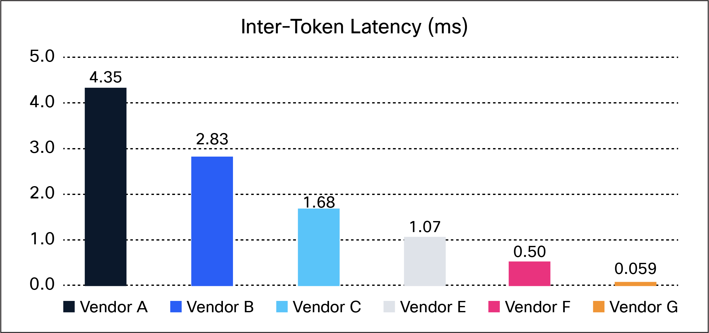
Evolution of inter-token latency across different hardware generations
It clearly shows how innovation is driving ITL down as new generations of inference hardware are developed, and we may expect the trend to continue in the upcoming years, as ITL is a major factor on the overall perceived latency.
But considering this, where is network latency here? Where does it fit or how relevant is it, if at all? This is a key question that we network engineers are interested in solving.
The relevance (or lack thereof) of WAN Network latency in AI Inference
It is obvious that, today, network latency is largely irrelevant in the end-to-end inference latency. When an inference may take probably up to a few seconds to complete, whether network latency is 10, 50, or 100ms is negligible.
However, we are entering into an era where many of the use cases or applications will be Agentic AI-based. One of the key implications of this is that a user request may result in tens or even hundreds of requests to an LLM to be completed. With that level of "chattiness," network latency may start playing a more relevant role. Let's see if that is true.
Let's suppose a scenario where an AI Agent needs to interact 100 times with an LLM to deliver a response to a user (while it may seem a large number, it is not so much in reality).
For analytical clarity, we separate network latency from TTFT, although in practice TTFT already includes part of the network round-trip time.
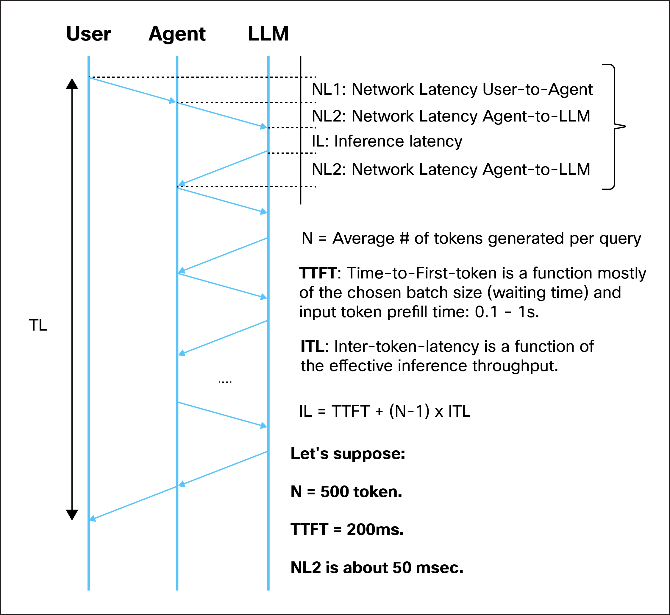
Latency components for an Agentic workflow
Essentially, the total latency perceived by the user (TL) is going to be influenced by the network latency associated to each communication segment plus the time it takes to complete inference (IL) for each LLM request.
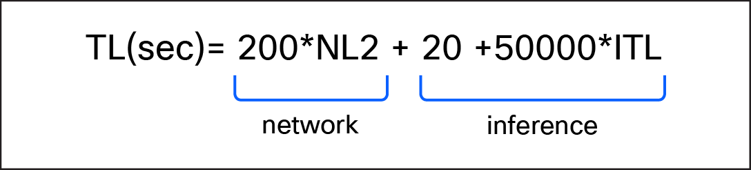
Considering the above numbers proposed as example, the Total Latency (TL) would follow this formula:
TL: Total Latency = 2 * NL1 + 100* (2*NL2 + IL) ≈ 200*NL2 + 100*TTFT + 100*N*ITL
Total user experience latency
We can group some of the terms and obtain a more simplified view that contains a network component and an inference component.
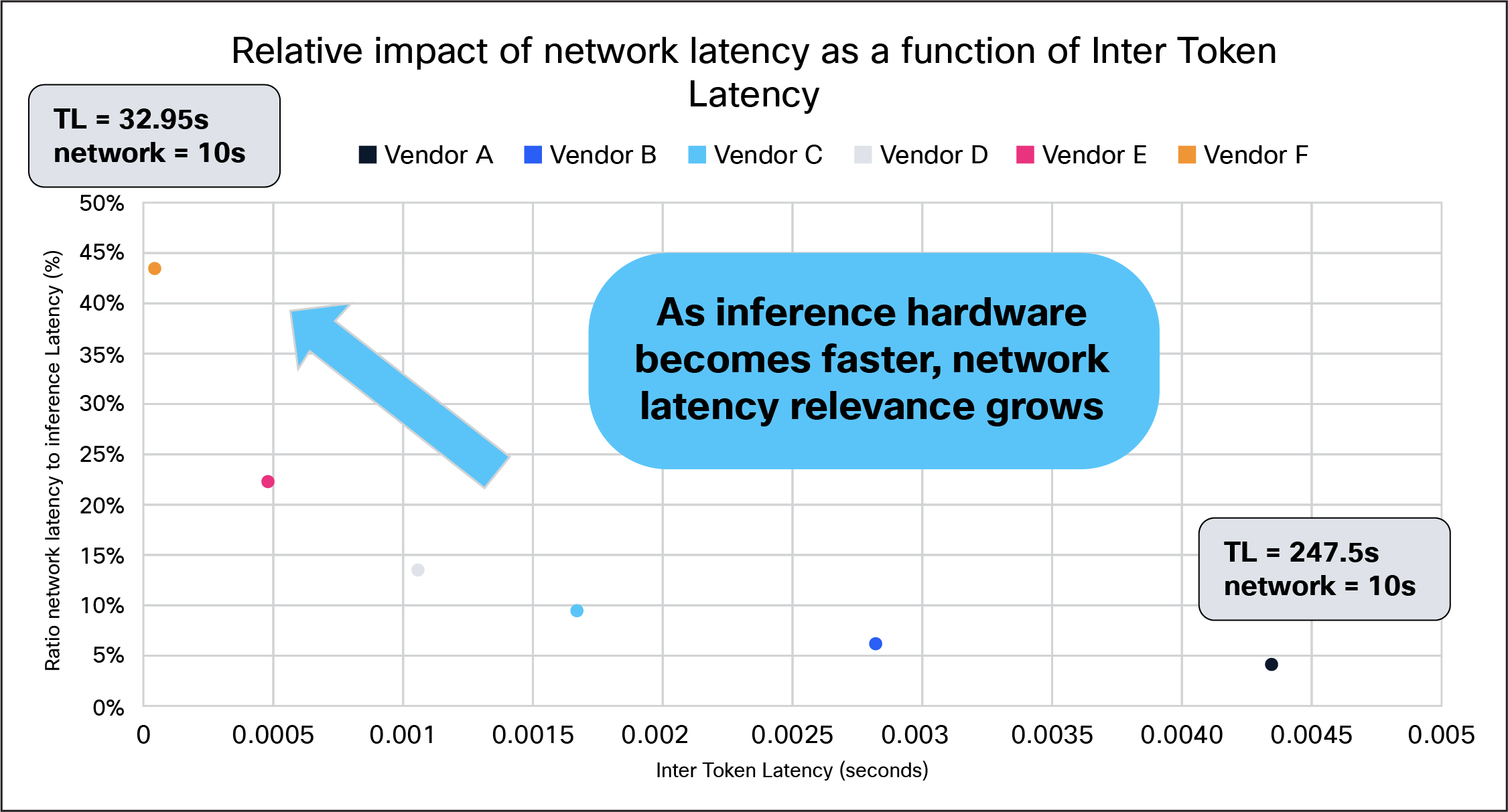
At this point, we still need to answer the key question: How relevant is the network component in this equation? One way to evaluate it is to compute the ratio between the network contribution above and the inference contribution. We are going to assume for this example that network latency between the agent and the LLM (NL2) is 50 msec.
Using the above formulas, and the various values of ITL that we have obtained earlier from the different inference hardware generations, we can see the following:
Network latency component versus inference latency component
For most of the current generations of inference hardware, the contribution of network latency compared to inference latency is a very low percentage, 10% or below. This basically means that as of today, in general, whether network latency is 50ms, or 40ms, or 20ms is going to have a minimal impact.
On the other hand, with the latest and fastest technologies, which can be also an indicator of where ITL may be in the next two or three years, network latency becomes 25% or even 45% of the inference latency, which then becomes a much more relevant contributor to the total latency perceived.
What this means in practice is, as inference hardware speed improves, network latency becomes much more relevant, and so does therefore the need to do inference in a more distributed way, closer to the users.
This clearly represents a heads-up for Service Providers, AI Inference will need to happen within much lower latency boundaries than where it is happening today, and this is an opportunity that should not be missed.
Conclusion: The Prompt as a Distributed Flow
A prompt may look like a simple interaction between a user and an AI assistant, but as we have seen, its journey is anything but simple. From the moment it is typed, a prompt becomes a distributed workload that traverses multiple domains: IP networks, API control planes, CPU-based preprocessing systems, and highly optimized GPU fabrics.
At its core, LLM inference is not a monolithic “AI operation.” It is a tightly orchestrated pipeline that combines:
● Network transport, to deliver and route requests
● CPU-based processing, to parse, tokenize, and schedule workloads
● GPU execution, to perform large-scale parallel computation
● High-performance interconnects, to enable multi-GPU coordination
● Streaming systems, to deliver responses in real time
For network engineers, this should feel familiar. The lifecycle of a prompt resembles the lifecycle of a flow in a modern distributed network:
● It is routed based on policy
● It is queued and scheduled under load
● It traverses multiple domains with different latency characteristics
● It relies on state (KV cache) to maintain continuity
● And it is ultimately delivered as a real-time stream
One of the most important insights is the existence of two distinct but interconnected fabrics:
● The request network (north-south), based on IP, TCP, and TLS
● The GPU fabric (east-west), based on NVLink, InfiniBand or Ethernet, and RDMA
Understanding where one ends and the other begins is key to reasoning about performance, scaling, and failure modes.
From a latency perspective, today’s systems are still largely dominated by compute — particularly the prefill phase and batching delays. However, this is changing rapidly. As inference hardware continues to improve and inter-token latency drops, network latency will become an increasingly significant component of the overall experience, especially in agentic workflows where dozens or hundreds of LLM interactions may be chained together.
This shift has important implications:
● Inference will need to move closer to the user
● Distributed inference architectures will become more prevalent
● Service providers will play a critical role in enabling low-latency AI infrastructure
In other words, AI inference is not just a compute problem anymore — it is becoming a networking problem again.
And for those who understand networks, that is not a challenge — it is an opportunity.
Javier Antich
CTO Office @ Provider Connectivity – Cisco