ACI Multi-Pod White Paper
Available Languages
Bias-Free Language
The documentation set for this product strives to use bias-free language. For the purposes of this documentation set, bias-free is defined as language that does not imply discrimination based on age, disability, gender, racial identity, ethnic identity, sexual orientation, socioeconomic status, and intersectionality. Exceptions may be present in the documentation due to language that is hardcoded in the user interfaces of the product software, language used based on RFP documentation, or language that is used by a referenced third-party product. Learn more about how Cisco is using Inclusive Language.
The ever-increasing adoption of ACI as pervasive fabric technology makes the need of interconnecting separate ACI fabrics very common for Enterprise and Service Providers. This is due to the fact that various business requirements (business continuance, disaster avoidance, etc.) lead to the deployment of separate Data Center fabrics that need to be interconnected with each other. As it will be clarified below, depending on the chosen deployment option, those fabrics may take the name of “Pods” or “Sites”.
Note: To best understand the design presented in this document, the reader should have basic knowledge of Cisco ACI and how it works and is designed for operation in a single site. For more information, see the Cisco ACI white papers available at the link below:
https://www.cisco.com/c/en/us/solutions/data-center-virtualization/application-centric-infrastructure/white-paper-listing.html.
Figure 1 highlights different design options for interconnecting ACI fabrics.
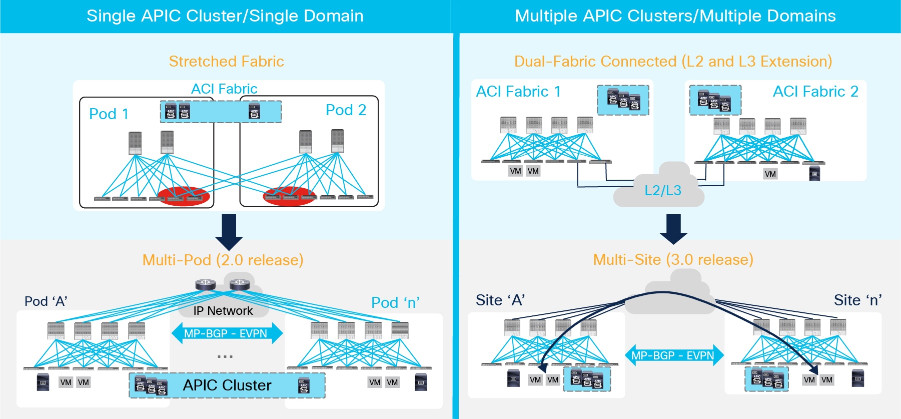
Design Option for Interconnecting ACI Fabrics
As highlighted above, there are two separate families of solutions:
1. Single APIC Cluster/Single Domain: Under this family we find the ACI Stretched Fabric and its natural evolution named Multi-Pod, which is the main focus of this paper. Both models leverage a single APIC controller cluster representing the single point of management and policy definition for the entire network, independently from the number of separate ACI fabrics (Pods) compounding it.
Note: For more information on ACI Stretched Fabric please refer to:
https://www.cisco.com/c/en/us/td/docs/switches/datacenter/aci/apic/sw/kb/b_kb-aci-stretched-fabric.html.
Those design options are usually fulfilling the requirements of interconnecting Data Centers deployed in Active/Active fashion, so to offer the freedom of deploying the various application components across separate Pods. The entire network hence runs as a single large fabric from an operational perspective; however, ACI Multi-Pod introduces specific enhancements to isolate as much as possible the failure domains between Pods, contributing to increase the overall design resiliency. This is achieved by running separate instances of fabric control planes (IS-IS, COOP, MP-BGP) across Pods.
At the same time, the tenant change domain is common for all the Pods, since a configuration or policy definition applied to any of the APIC nodes would be propagated to all the Pods managed by the single APIC cluster. This behavior is what greatly simplifies the operational aspects of the solution.
2. Multiple APIC Cluster/Multiple Domains: Those deployment options are characterized by having an independent APIC cluster managing each interconnected ACI network. This provides complete ‘air-gap’ between the ACI fabrics, since configuration and policy definitions can be scoped independently. The typical use case for this type of solutions is disaster recovery: a secondary DC site is deployed to be able to recover applications after a major failure that brought down the principal site(s) where the applications were initially running.
The first possible designs is shown in the top right corner of Figure 1 and named Dual-Fabric. This deployment model leverages more traditional Layer 2 and Layer 3 Data Center Interconnect (DCI) technology options to connect separate ACI fabrics. Dual-Fabric design represents a disjointed domain from a policy perspective, as there is the requirement to reclassify endpoint traffic (Layer 2 or Layer 3) at the point of entrance of each ACI fabric and to ensure the same configuration is created in each APIC domain for providing a consistent end-to-end policy application.
In order to overcome some of the challenges of the Dual-Fabric design, starting from ACI release 3.0 Cisco delivered the architecture representing the evolution of the Dual-Fabric option and named “ACI Multi-Site”. For more information on ACI Multi-Site please refer to the paper available at the link below:
Note: When operating more than one ACI fabric, it is highly recommended to deploy Multi-Site instead of interconnecting multiple individual ACI fabrics to each other via leaf switches (dual-fabric design). Although the latter option may have been one of the only ways prior to these features, it is currently not supported because no validations and quality assurance tests are performed in this topology for many other new features, such as L3 multicast. Hence, although ACI has a feature called Common Pervasive Gateway for interconnecting ACI fabrics prior to Multi-Site, it is highly recommended to design a new ACI fabric with Multi-Site instead when there is a requirement to interconnect separate APIC domains.
As previously mentioned, this document is fully focused on the ACI Multi-Pod design option that has been released as part of ACI 2.0 Software release. Before describing more in detail the various functional components of the solution, it is required to provide a short overview of ACI Multi-Pod and clarify what are some of the typical business problems it allows to solve.
ACI Multi-Pod represents the natural evolution of the original ACI Stretched Fabric design and allows to interconnect and centrally manage separate ACI networks (Figure 2).
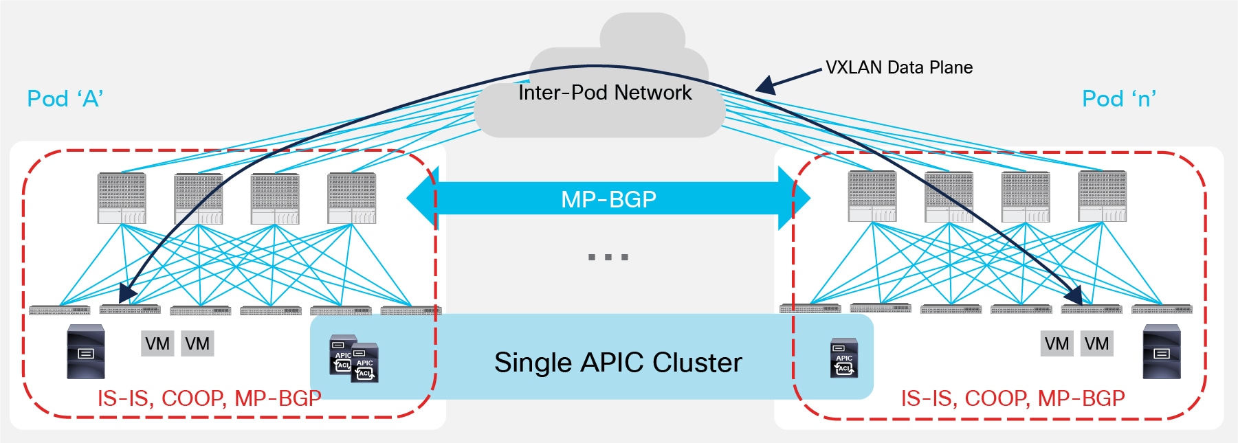
ACI Multi-Pod Solution
As it was discussed in the introduction, ACI Multi-Pod is part of the “Single APIC Cluster/Single Domain” family of solutions as a single APIC cluster is deployed to manage all the different ACI networks that are interconnected. Those separate ACI networks are named “Pods” and each of them looks like a regular two-tiers spine-leaf topology. The same APIC cluster can manage several Pods and to increase the resiliency of the solution the various controller nodes that make up the cluster can be deployed across different Pods (as it will be discussed in greater detail in the “APIC Cluster Deployment Considerations” section).
The deployment of a single APIC cluster simplifies the management and operational aspects of the solution, as all the interconnected Pods essentially function as a single ACI fabric: created tenants configuration (VRFs, Bridge Domains, EPGs, etc.) and policies are made available across all the Pods, providing a high degree of freedom for connecting endpoints to the fabric. For example, different workloads that are part of the same functional group (EPG), like Web servers, can be connected to (or moved across) different Pods without having to worry about provisioning configuration or policy in the new location. At the same time, seamless Layer 2 and Layer 3 connectivity services can be provided between endpoints independently from the physical location where they are connected and without requiring any specific functionality from the network interconnecting the various Pods.
Even if the various Pods are managed and operated as a single distributed fabric, Multi-Pod offers the capability of increasing failure domain isolation across Pods through separation of the fabric control plane protocols. As highlighted in Figure 2, different instances of IS-IS, COOP and MP-BGP protocols run inside each Pod, so that faults and issues with any of those protocols would be contained in the single Pod and not spread across the entire Multi-Pod fabric. This is a property that clearly differentiates Multi-Pod from the Stretched Fabric approach and makes it the recommended design option going forward.
From a physical perspective, the different Pods are interconnected by leveraging an “Inter-Pod Network” (IPN). Each Pod connects to the IPN through the spine nodes; the IPN can be as simple as a single Layer 3 device, or can be built with a larger Layer 3 network infrastructure, as it will be clarified in the “Inter-Pod Connectivity Deployment Considerations” section.
Nonetheless, the IPN must simply provide basic Layer 3 connectivity services, allowing for the establishment across Pods of spine-to-spine and leaf-to-leaf VXLAN tunnels. It is the use of the VXLAN overlay technology in the data-plane that provides seamless Layer 2 and Layer 3 connectivity services between endpoints, independently from the physical location (Pod) where they are connected. Details about endpoint data-plane communication across Pods will be presented in the “Inter-Pods VXLAN Data Plane” section.
Finally, running a separate instance of the COOP protocol inside each Pod implies that information about discovered endpoints (MAC, IPv4/IPv6 addresses and their location) is only exchanged using COOP as a control plane protocol between the leaf and spine nodes locally deployed in each Pod. Since ACI Multi-Pod functions as a single fabric, it is key to ensure that the databases implemented in the spine nodes across Pods have a consistent view of the endpoints connected to the fabric; this requires the deployment of an overlay control plane running between the spines and used to exchange endpoint reachability information. As shown in Figure 2, Multi-Protocol BGP has been chosen for this function. This is due to the flexibility and scalability properties of this protocol and its support of different address-families (like EVPN and VPNv4) allowing the exchange of Layer 2 and Layer 3 information in a true multi-tenant fashion. More considerations about the use of MP-BGP as overlay control plane will be found in the “Inter-Pods MP-BGP Control Plane” section.
ACI Multi-Pod Use Cases and Supported Topologies
There are two main use cases for the deployment of ACI Multi-Pod and their substantial difference is the physical location where the different Pods are deployed.
● Multiple Pods deployed in the same physical data center location: this scenario is shown in Figure 3 below.
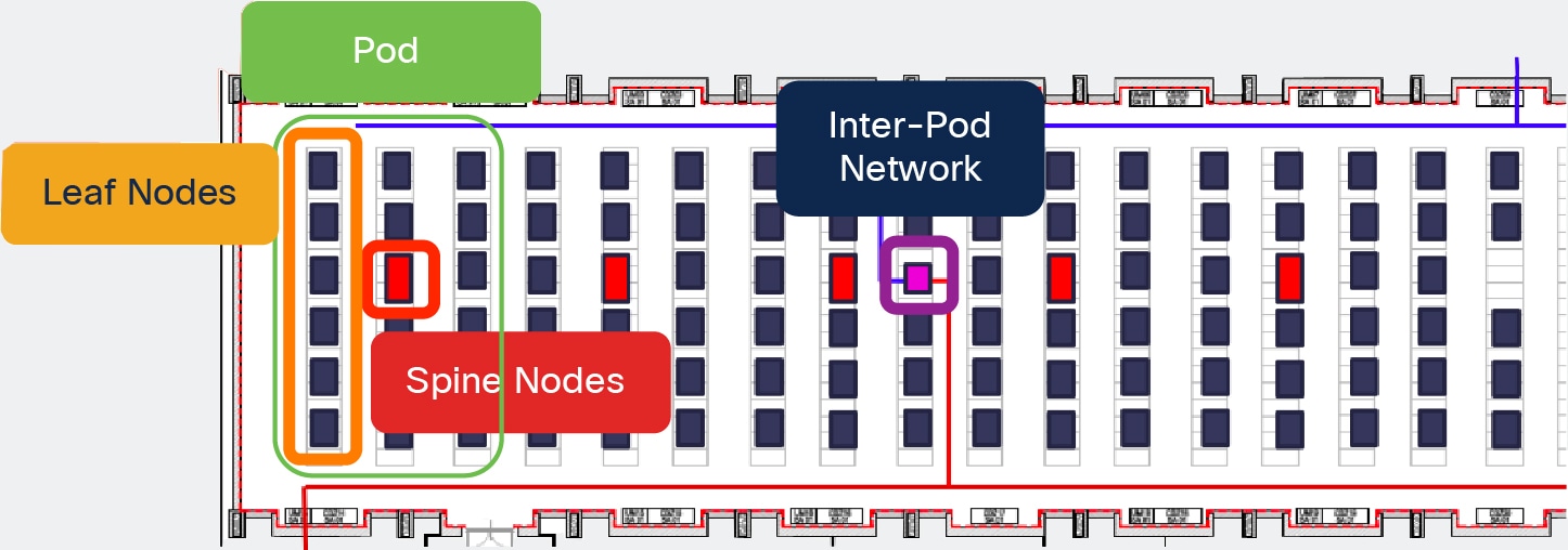
Multiple Pods in the Same Physical Data Center
The creation of multiple Pods could be driven, for example, by the existence of a specific cabling layout already in place inside the data center. In the example above, top-of-rack switches are connected to middle-of-row devices (red rack) and the various middle-of-row switches are aggregated by core devices (purple rack). Such cabling layout does not allow for the creation of a typical two-tier leaf-spine topology; the introduction of ACI Multi-Pod permits to interconnect all the devices in a three tier topology and centrally manage them as a single fabric.
Another scenario where multiple Pods could be deployed in the same physical data center location is when the requirement is the creation of a very large fabric. In that case it may be desirable to divide the large fabric in smaller Pods to benefit of the failure domain isolation provided by the Multi-Pod approach.
● The most common use case for the deployment of ACI Multi-Pod is the one captured in Figure 4, where the different Pods represent geographically dispersed data centers.
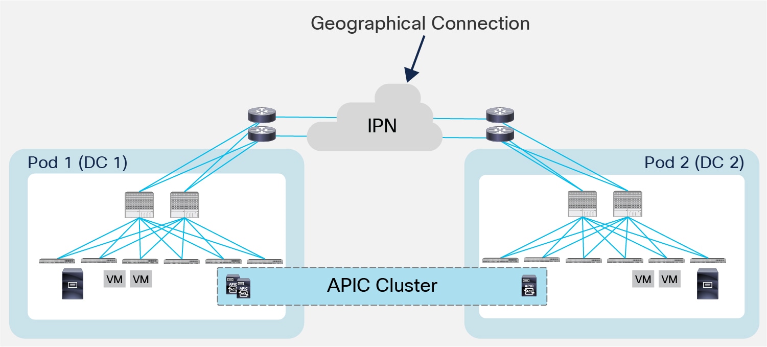
Multiple Pods across Different Data Center Locations
The deployment of Multi-Pod in this case ensures to meet the requirement of building Active/Active Data Centers, where different application components can be freely deployed across Pods. The different data center networks are usually deployed in relative proximity (metro area) and are interconnected leveraging point-to-point links (dark fiber connections or DWDM circuits).
Based on the use cases described above, Figure 5 shows the supported Multi-Pod topologies.
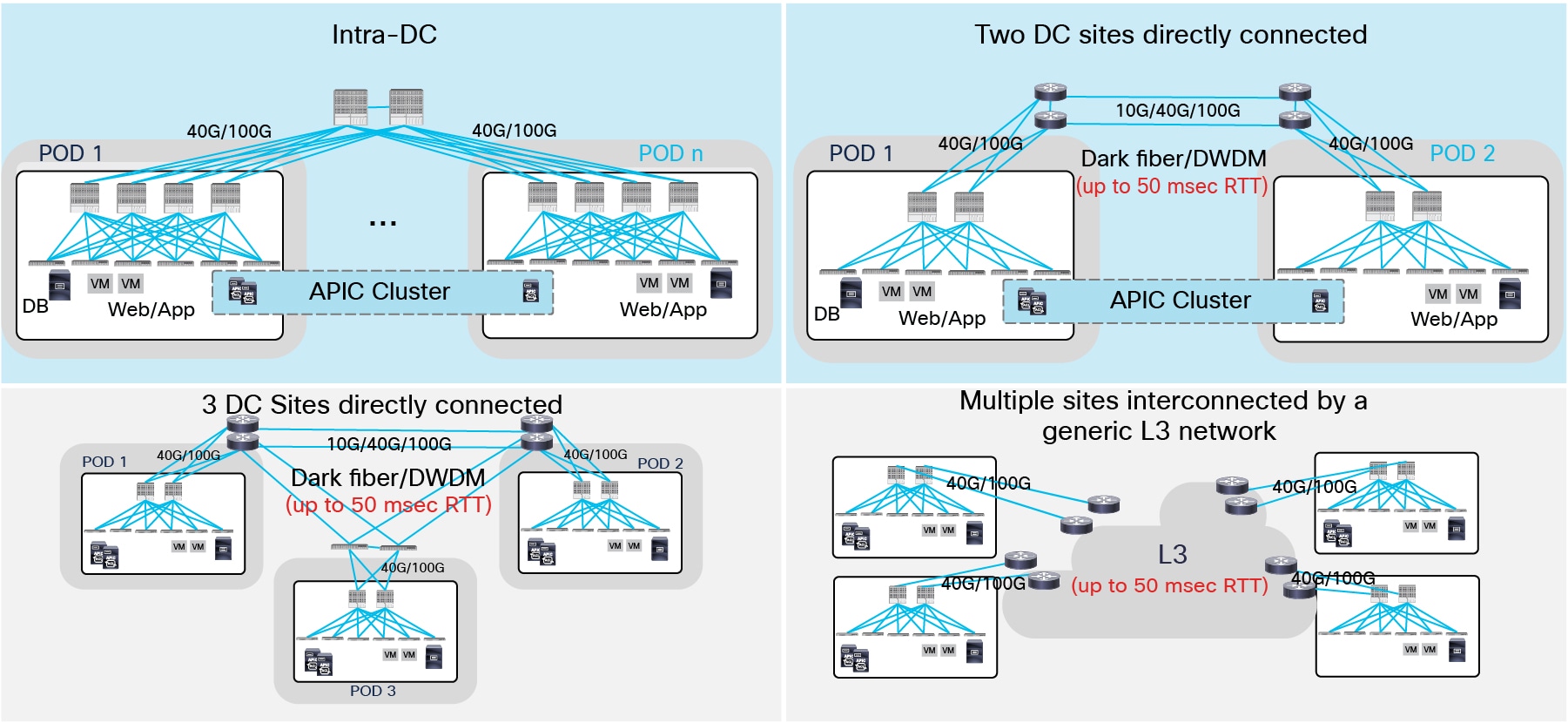
Multi-Pod Supported Topologies
In the top left corner is shown the topology matching the first use case. Since the Pods are locally deployed (in the same data center location), a pair of centralized IPN devices can be use to interconnect the different Pods. Those IPN devices must potentially support a large number of 40G/100G interfaces, so a couple of modular switches are likely to be deployed in that role.
The other three topologies apply instead to scenarios where the Pods are represented by separate physical data centers. Starting from ACI release 2.3, the maximum latency supported between Pods is 50 msec RTT, which roughly translates to a geographical distance of up to 2500 miles. Also, the IPN network is often be represented by point-to-point links (dark fibers or DWDM circuits); in specific cases, a generic Layer 3 infrastructure (for example an MPLS network) can also be leveraged as IPN as long as it satisfies the requirements described in the “Inter-Pod Connectivity Deployment Considerations” section.
Note: Beginning with Cisco APIC Release 5.2(3), the ACI Multi-Pod architecture is enhanced to support connecting the spines of two Pods directly with back-to-back ("B2B") links. With this solution, called Multi-Pod Spines Back-to-Back, the IPN requirement can be removed for small ACI Multi-Pod deployments. Multi-Pod Spines Back-to-Back also brings operational simplification and end-to-end fabric visibility, as there are no external devices to configure. For more information, please refer to the paper at the link below: https://www.cisco.com/c/en/us/td/docs/dcn/aci/apic/kb/cisco-multipod-b2b.html
ACI Multi-Pod Scalability Considerations
Before discussing more in detail the various functional components of the ACI Multi-Pod solution, it is important to reiterate how this model functionally represents a single fabric. As discussed, this is a very appealing aspect of the solution, as it facilitates operating such infrastructure. At the same time, this enforces some scalability limits since all the deployed nodes must be managed by a single APIC controller cluster.
The bulleted list below describes the scalability figures for ACI Multi-Pod based on what supported in the 5.2 release.
● Maximum number of Pods: 12
Note: Support for 12 Pods is available from ACI release 3.0 when deploying a 7 nodes APIC cluster.
● Maximum number of Leaf nodes across all Pods:
◦ 500 with a 7 nodes APIC cluster (from ACI release 4.2(4))
◦ 300 with a 5 nodes APIC cluster
◦ 200 with a 4 nodes APIC cluster (from ACI release 4.0(1))
◦ 80 with a 3 nodes APIC cluster
● Maximum number of Leaf nodes per Pod: 400 (from ACI release 4.2(4))
● Maximum number of Spine nodes per Pod: 6
Note: It is recommended to consult the ACI release notes for updated scalability figures and also for information on other scalability parameters not listed above.
Inter-Pod Connectivity Deployment Considerations
The Inter-Pod Network (IPN) is connecting the different ACI Pods allowing for the establishment of Pod-to-Pod communication (also known as east-west traffic). In this function, the IPN basically represents an extension of the ACI fabric underlay infrastructure.
A common question is whether a minimum bandwidth is required between Pods that are part of the same Multi-Pod fabric. While technically the architecture can be fully functional, even when deploying a pair of 1G connections between Pods, it is obvious that the ideal amount of bandwidth mostly depends on the amount of east-west connectivity required. In any case, it is always recommended to prioritize at least the control-plane communication between spines of different Pods and the intra-cluster communication when deploying the APIC controller nodes across different Pods.
Another typical question is whether specific network devices should be deployed as IPN routers. The simple answer is that any device that can fulfill the requirements listed in the following paragraphs is perfectly suited for performing the IPN duties. However, the recommendation is to deploy, when possible, switches of the Cisco Nexus® 9200 family or switches of Cisco Nexus 9300 second-generation (or older) family (i.e., EX models or newer), as they are the ones most commonly found in production and also the ones more frequently validated in Cisco internal testing.
In order to perform those connectivity functions, the IPN must support few specific functionalities described below.
● Multicast support: In addition to unicast communication, east-west traffic also comprises Layer 2 multi-destination flows belonging to bridge domains that are extended across Pods. This type of traffic is usually referred to as BUM (Broadcast, Unknown Unicast and Multicast) and it is exchanged by leveraging VXLAN data plane encapsulation between leaf nodes.
Inside a Pod (or ACI fabric), BUM traffic is encapsulated into a VXLAN multicast frame and it is always transmitted to all the local leaf nodes. A unique multicast group is associated to each defined Bridge Domain and takes the name of Bridge Domain Group IP–outer (BD GIPo). Once received by the leafs, it is then forwarded to the connected devices that are part of that Bridge Domain or dropped depending on the type of BUM frame and on the specific Bridge Domain configuration.
The same behavior must be achieved for endpoints part of the same Bridge Domain that are connected to different Pods. In order to flood the BUM traffic across Pods, the same multicast group used inside the Pod is also extended through the IPN network. Those multicast groups should work in PIM Bidir mode and must be dedicated to this function (i.e. not used for other purposes, applications, etc.).
The main reasons for using PIM Bidir in the IPN network are:
1. Scalability: Since BUM traffic can be originated by all the leaf nodes deployed across Pods, the use of a different PIM protocol (like PIM ASM, for example) would results in the creation of multiple individual (S, G) entries on the IPN devices that may exceed the specific platform capabilities. With PIM Bidir, a single (*, G) entry must be created for a given BD, independently from the overall number of leaf nodes.
2. No requirement for data-driven multicast state creation: The (*, G) entries are created in the IPN devices as soon as a BD is activated in the ACI Multi-Pod fabric, independently from the fact there is an actual need to forward BUM traffic across Pods for that given BD. This implies that when the need to do so arises, the network will be ready to perform those duties, avoiding longer convergence time for the application caused for example in PIM ASM by the data-driven state creation.
3. It represents Cisco’s prescriptive, well-tested and hence recommended design option.
● DHCP relay support: One of the nice functionalities offered by the ACI Multi-Pod solution is the capability of allowing auto-provisioning of configuration for all the ACI devices deployed in remote Pods. This allows those remote Pods to join the Multi-Pod fabric with zero-touch configuration, as it normally happens to ACI nodes part of the same fabric (Pod). This functionality relies on the capability of the first IPN device connected to the spines of the remote Pod to relay DHCP requests generated from a new starting ACI spines toward the APIC node(s) active in the first Pod. More considerations about this zero-touch provisioning functionality can be found in the “Pod Auto-Provisioning” section.
● OSPF support: In the initial release of ACI Multi-Pod fabric, OSPFv2 is the routing protocol (in addition to static routing) supported on the spine interfaces connecting to the IPN devices.
● Increased MTU support: Since VXLAN data-plane traffic is exchanged between Pods, the IPN must ensure to be able to support an increased MTU on its physical connections, in order to avoid the need for fragmentation and reassembly. Before ACI release 2.2, the spine nodes were hard-coded to generate 9150B full-size frames for exchanging MP-BGP control plane traffic with spines in remote Pods. This mandated support for that 9150B MTU size across all IPN devices. From ACI release 2.2, a global configuration knob has been added on APIC to allow proper tuning of the MTU size of all the control plane packets generated by ACI nodes (leaf and spines), including inter-Pod MP-BGP control plane traffic. This essentially implies that the MTU support required in the IPN becomes solely dependent on the maximum size of frames generated by the endpoints connected to the ACI leaf nodes (that is, it must be 50B higher than that value).
● The spine interfaces are connected to the IPN devices through point-to-point routed interfaces. However, traffic originated from the spine interfaces is always tagged with an 802.1q VLAN 4 value, which implies the need to define and support Layer 3 sub-interfaces on both the spines and the directly connected IPN devices. It is hence critical to select IPN routers that allow to define multiple sub-interfaces on the same device using the same VLAN tag 4 and still functioning as separate point-to-point L3 links.
Note: The use of sub-interfaces on the ISN devices is only mandatory for the connections toward the spines.
● QoS considerations: As highlighted in Figure 6 below, traffic inside an ACI Pod can be separated in different classes of services.
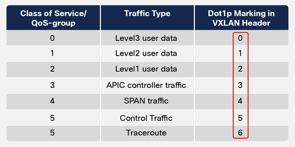
Intra-Pod Classes of Traffic
Each class of service is identified with a specific 802.1p (CoS) value in the outer Layer 2 header of the VXLAN encapsulated traffic routed inside the Pod. This information allows the spine and leaf nodes inside the Pod to perform proper traffic classification and prioritization.
In an ACI Multi-Pod deployment, two important considerations arise when discussing end-to-end QoS behavior:
1. First, since the IPN devices are external to the ACI fabric and are hence not managed by APIC, in many cases it may not be possible to assume that the 802.1p values are properly preserved across the IPN network. By default traffic received by the spines on the interfaces connecting to the IPN devices is classified to one of the classes of traffic shown in Fig. 6 based on the CoS value in the outer IP header of inter-pod iVXLAN traffic. This may lead to unexpected handling inside the fabric for traffic flows received from the IPN. As a consequence, the recommendation is to configure a proper CoS-to-DSCP mapping on APIC to ensure that traffic received on the spine nodes of a remote Pod can be reassigned to its proper class of service before being injected into the Pod based on the DSCP value in the outer IP header of inter-pod iVXLAN traffic, as shown in Figure 7 below.
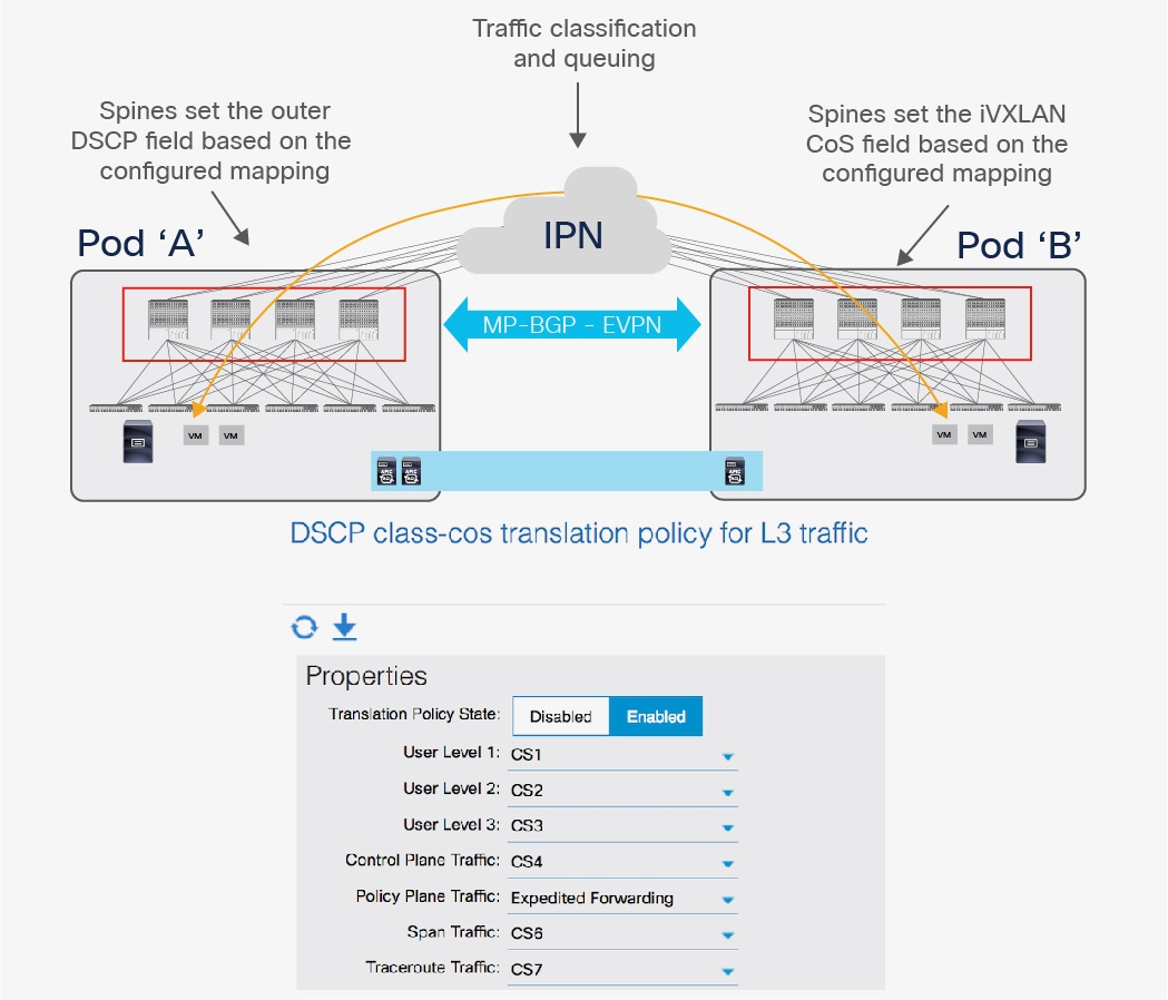
CoS-to-DSCP Mapping on the Spine Nodes
Note: Future ACI software release may allow to configure more user level classes (compared to the three supported at the time of writing of this paper). This won’t change the design recommendations and deployment considerations contained in this section.
2. The DSCP values set by the spine nodes before sending the traffic into the IPN network can then be used to differentiate and prioritize the different types of traffic. In the example above, Policy Plane Traffic (that is, communication between APIC nodes deployed in separate Pods) is marked as Expedited Forwarding (EF), whereas Control Plane Traffic (that is, OSPF and MP-BGP packets) is marked as CS4. The IPN devices can be configured to prioritize those two types of traffic to ensure that the policy and control plane remains stable also in scenarios where a large amount of east-west user traffic is required across Pods.
Note: The configuration required on the IPN devices to classify and prioritize the different types of traffic depends on the specific platforms deployed and is out of the scope of this paper.
As previously mentioned, the Inter-Pod Network represents an extension of the ACI infrastructure network, ensuring VXLAN tunnels can be established across Pods for allowing endpoints communication.
Inside each ACI Pod, IS-IS is the infrastructure routing protocol used by the leaf and spine nodes to peer with each other and exchange IP information for locally defined loopback interfaces (usually referred to as VTEP addresses). During the auto-provisioning process for the nodes belonging to a Pod, the APIC assigns one (or more) IP addresses to the loopback interfaces of the leaf and spine nodes part of the Pod. All those IP addresses are part of an IP pool that is specified during the boot-up process of the first APIC node and takes the name of ‘TEP pool’.
In a Multi-Pod deployment, each Pod is assigned a separate and not overlapping TEP pool, as shown in Figure 8.
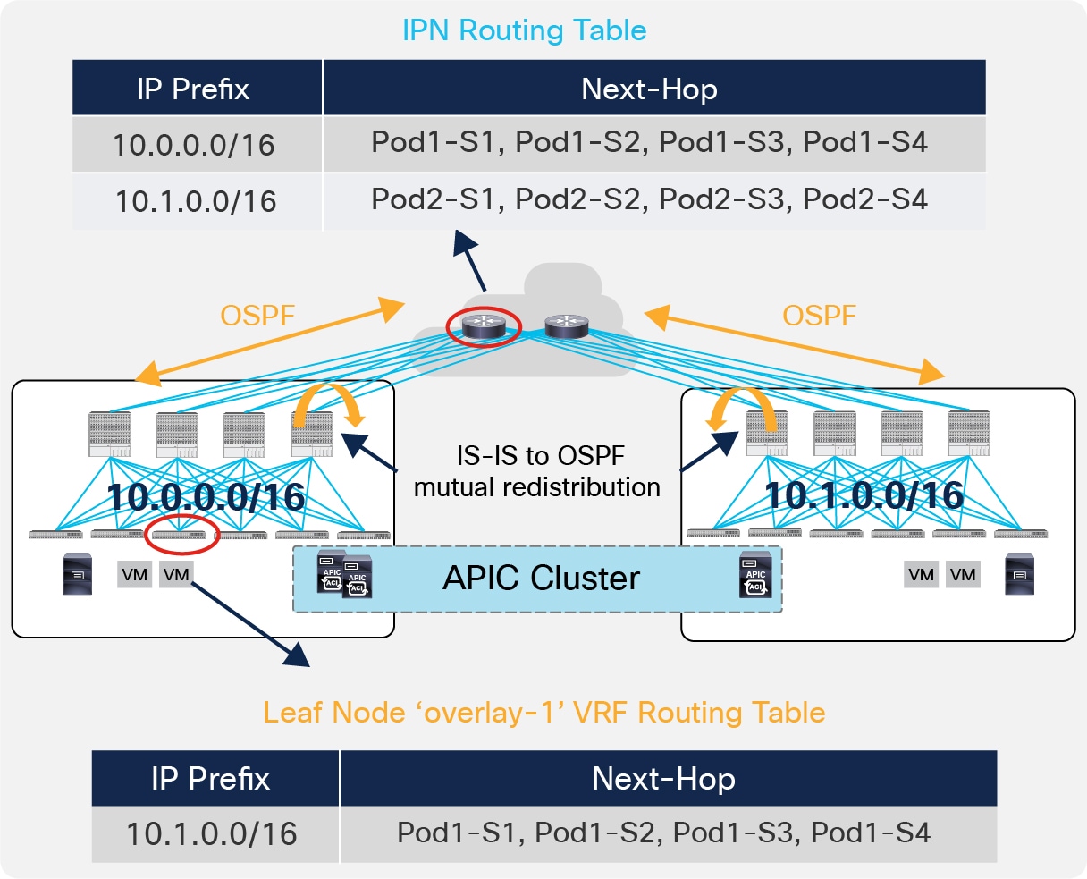
IPN Control Plane
The spines in each Pod establish OSPF peerings with the directly connected IPN devices to be able to send out the TEP pool prefix for the local Pod. As a consequence, the IPN devices install in their routing tables equal cost routes for the TEP pools valid in the different Pods. At the same time, the TEP-Pool prefixes relative to remote Pods received by the spines via OSPF are redistributed into the IS-IS process of each Pod so that the leaf nodes can install them in their routing table (those routes are part of the ‘overlay-1’ VRF representing the infrastructure VRF).
Note: Nonetheless, the spines also send few host route addresses to the IPN, associated to specific loopback addresses defined on the spines. This is required to ensure that traffic destined to those IP addresses can be delivered from the IPN directly to the right spine where they are defined (i.e. not following equal cost paths that may lead to a different spine). No host routes for leaf nodes loopback interfaces should ever be sent into the IPN and this ensures to keep the routing table of the IPN devices very lean independently from the total number of deployed leaf nodes.
The fact that an OSPF peering is required between the spines and the IPN devices (at the time of writing of this document, OSPF is the only supported protocol for this function) does not mean that OSPF must be used across the entire IPN infrastructure.
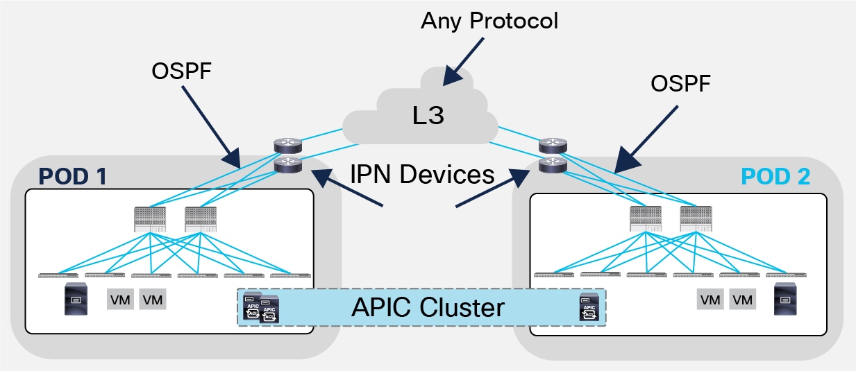
Support of Any Protocol in the IPN
Figure 9 highlights this design point; this could be the case when the IPN is a generic Layer 3 infrastructure interconnecting the Pods (like an MPLS network, for example) and a separate routing protocol could be used inside that Layer 3 network. Mutual redistribution would then be needed with the process used toward the spines.
The use of VXLAN as overlay technology allows providing Layer 2 connectivity services between endpoints that may be deployed across Layer 3 network domains. Those endpoints must be able of sending and receiving Layer 2 multi-destination frames (BUM traffic), as they are logically part of the same Layer 2 domain. BUM traffic can be exchanged across Layer 3 network boundaries by encapsulating it into VXLAN packets addressed to a multicast group, so to leverage the network for traffic replication services.
Figure 10 shows the use of multicast inside the ACI infrastructure to deliver multi-destination frames to endpoints part of the same Bridge-Domain (BD).
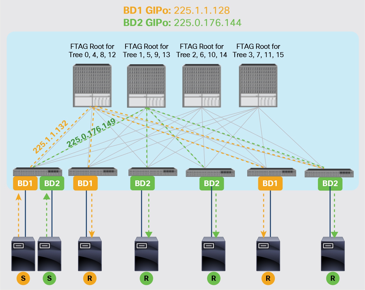
Use of Multicast for BUM replication in the ACI Infrastructure
Each Bridge Domain has associated a separate multicast group (named ‘GIPo’) to ensure granular delivery of multi-destination frames only to the endpoints that are part of a given Bridge-Domain.
Note: As shown in figure above, in order to fully leverage different equal cost paths also for the delivery of multi-destination traffic, separate multicast trees are built and used for all the defined Bridge Domains.
A similar behavior must be achieved when extending the Bridge Domain connectivity across Pods. This implies the need to extend multicast connectivity through the IPN network, which is the reason why those devices must support PIM Bidir.
Multi-destination frames generated by an endpoint part of a BD are encapsulated by the leaf node where the endpoint is connected and need then to transit across the IPN network to reach remote endpoints part of the same BD. For this to happen, the spines must perform two basic functions:
● Forward received multicast frames toward the IPN devices to ensure they can be delivered to the remote Pods.
● Send IGMP joins toward the IPN network every time a new Bridge Domain is activated in the local Pod, to be able to receive BUM traffic for that BD originated by an endpoint connected to a remote Pod.
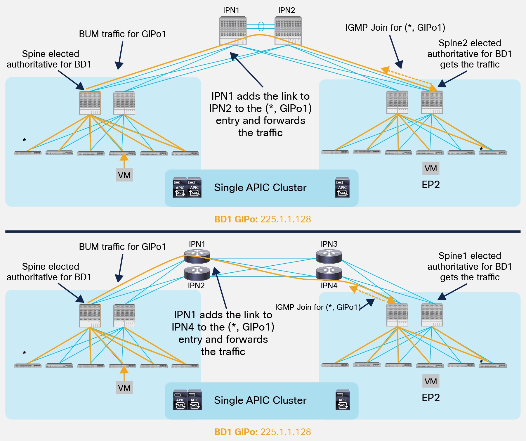
For each Bridge Domain, one spine node is elected as the authoritative device to perform both functions described above (the IS-IS control plane between the spines is used to perform this election). As shown in Figure 11, the elected spine will select a specific physical link connecting to the IPN devices to be used to send out the IGMP join (hence to receive multicast traffic originated by a remote leaf) and for forwarding multicast traffic originated inside the local Pod.
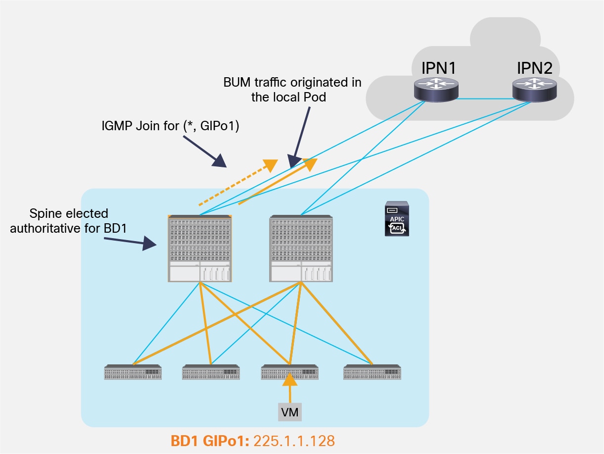
IGMP Join and BUM Forwarding on the Designated Spine
Note: If case of failure of the designated spine, a new one will be elected to take over that role.
As a result, the end-to-end BUM forwarding between endpoints part of the same Bridge Domain and connected in separate Pods happens as shown in figure below.
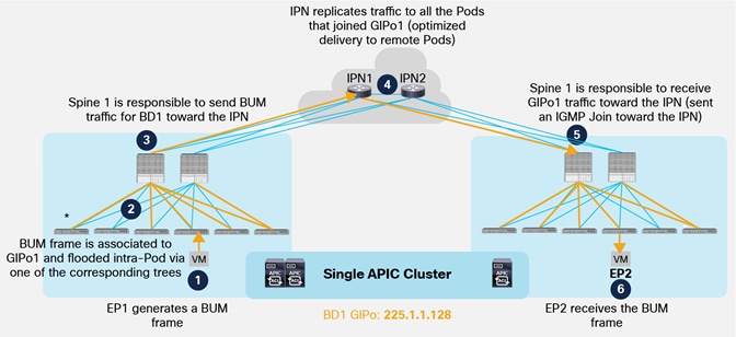
Delivery of BUM Traffic between Pods
1. EP1 belonging to BD1 originates a BUM frame.
2. The frame is encapsulated by the local leaf node and destined to the multicast group GIPo1 associated to BD1. As a consequence, it is sent along one of the multi-destination tree assigned to BD1 and reaches all the local spine and leaf nodes where BD1 has been instantiated.
3. Spine 1 is responsible for forwarding BUM traffic for BD1 toward the IPN devices, leveraging the specific link connected to IPN1.
4. The IPN device receives the traffic and performs multicast replication toward all the Pods from which it received an IGMP Join for GIPo1. This ensures that BUM traffic is sent only to Pods where BD1 is active (i.e. there is at least an endpoint actively connected in the Bridge Domain).
5. The spine that sent the IGMP Join toward the IPN devices receives the multicast traffic and forwards it inside the local Pod along one of the multi-destination trees associated to BD1. All the leafs where BD1 has been instantiated receive the frame.
6. The leaf where EP2 is connected also receives the stream, decapsulates the packet and forwards it to EP2.
An important design consideration should be made for the deployment of the Rendezvous Point (RP) in the IPN network. The role of the RP is important in a PIM Bidir deployment, as all multicast traffic in Bidir groups vectors toward the bidir RPs, branching off as necessary as it flows upstream and/or downstream. This implies that all the BUM traffic exchanged across Pods would be sent through the same IPN device acting as RP for the 225.0.0.0/15 default range used to assign multicast groups to each defined Bridge Domain. A possible design choice to balance the work load across different RPs consists in splitting the range and configure the active RP for each sub-range on a separate IPN devices, as shown in the simple example in Figure 13.
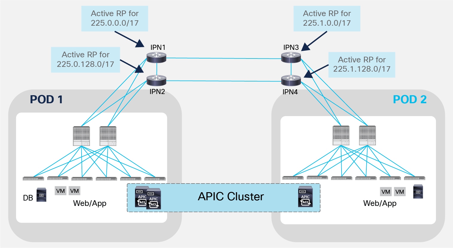
Multiple Active RPs Deployment
It is also important to notice that when deploying PIM Bidir, at any given time it is only possible to have an active RP for a given multicast group range (for example IPN1 is the only active RP handling the 225.0.0.0/17 multicast range). RP redundancy is hence achieved by leveraging the “Phantom RP” configuration, as described in the “ACI Multi-Pod Configuration” documents at the link below: https://www.cisco.com/c/en/us/solutions/collateral/data-center-virtualization/application-centric-infrastructure/white-paper-c11-739714.html.
Spines and IPN Connectivity Considerations
Several considerations arise when discussing how to interconnect the spines deployed in a Pod to the IPN devices, or how the IPN devices deployed in separate Pods should be connected together.
The first point to clarify is that it is not a mandatory requirement to connect every spine deployed in a Pod to the IPN devices.
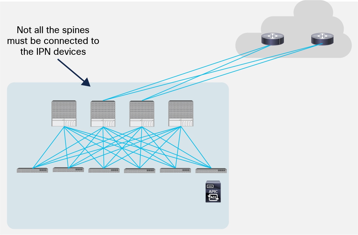
Partial Mesh Connectivity between Spines and IPN
Figure 14 shows a scenario where only two of the 4 spines are connected to the IPN devices. There are not functional implications for unicast communication across sites, as the local leaf nodes encapsulating traffic to a remote Pod would always prefer the paths via the spines that are actively connected to the IPN devices (based on IS-IS routing metric). At the same time, there are no implications either for the BUM traffic that needs to be sent to remote Pods, as only the spine nodes that are connected to the IPN devices are considered for being designated as responsible to send/receive traffic for a GIPo (via IS-IS control plane exchange).
Another consideration is about the option of connecting the spines belonging to separate Pods with direct back-to-back links, as shown in Figure 15.
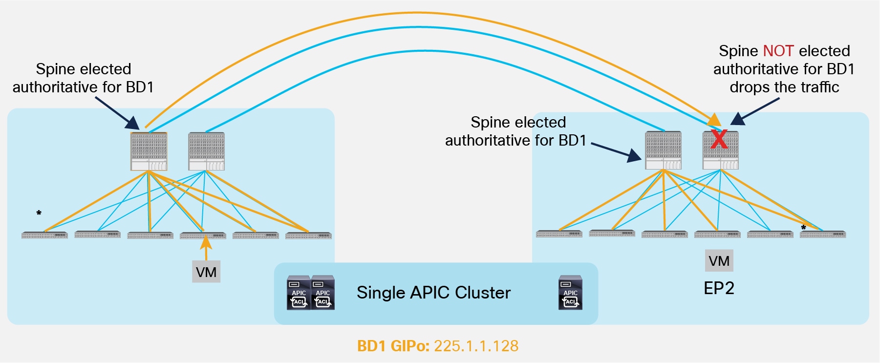
Direct Back-to-Back Links between Spines in Separate Pods (NOT Supported)
As shown above, direct connectivity between spines may lead to the impossibility of forwarding BUM traffic across Pods, in scenarios where the directly connected spines in separate Pods are not both elected as designated for a given Bridge Domain. As a consequence, the recommendation is to always deploy at least a Layer 3 IPN device (a pair for redundancy) between Pods.
It is important to point out that a similar behavior could be achieved also when connecting the spines to the IPN devices. Consider for example the topologies in Figure 16.
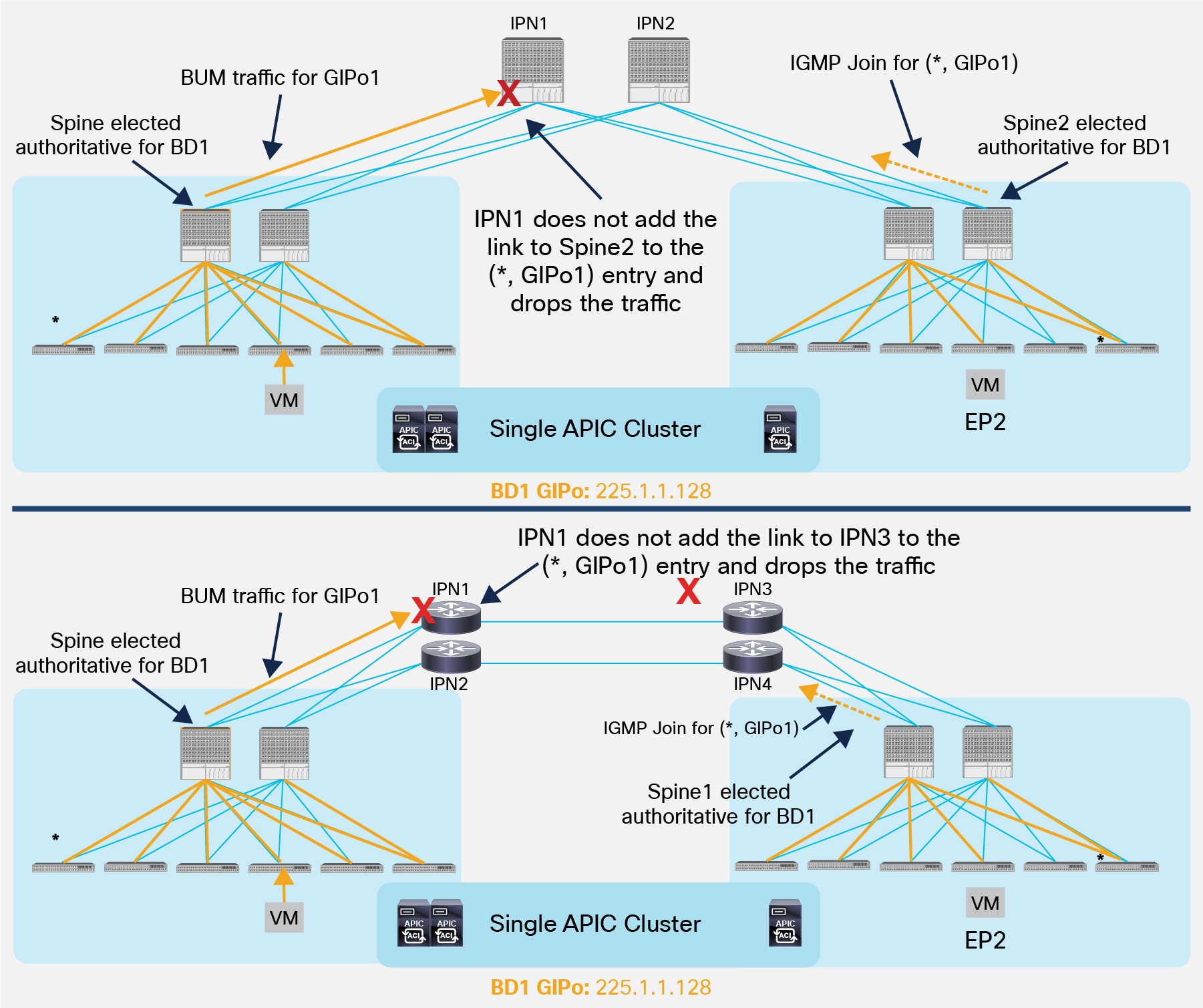
Issues in Sending BUM Traffic across Pods (NOT Supported)
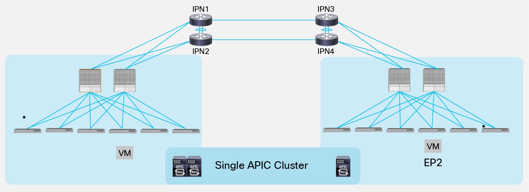
Both scenarios above highlight a case where the designated spines in Pod1 and Pod2 (for GIPo1) sends the BUM traffic and the IGMP Join for that group to two different IPN nodes that do not have a physical path between them. As a consequence, the IPN devices won’t have proper (*, G) state and the BUM communication would fail. To avoid this from happening, the recommendation is to always ensure that there is a physical path interconnecting all the IPN devices, as shown in Figure 17.
Establishing a Physical Path between IPN Devices
Note: The full mesh connections in the bottom scenario could be replaced by a Layer 3 port-channel connecting the local IPN devices. This would be useful to reduce the number of required geographical links, as shown in Figure 18 below.
L3 Port-Channels Connecting Local IPN Devices
Establishing the physical connections between IPN devices as shown in the previous figures guarantees that each IPN router has a physical path toward the PIM Bidir active RP. It is critical to ensure that the preferred path between two IPN nodes does not go through the spine devices, because that would break multicast connectivity (since the spines are not running the PIM protocol). For example, still referencing figure 18 above, if the Layer 3 port-channel connecting the two IPN devices is created by bundling 10G interfaces, the preferred OSPF metric for the path between IPN1 and IPN2 could indeed steer the traffic through one of the spines in Pod1. In order to solve the issue, it is recommended to deploy links of consistent speed (10/40/100G) for connecting local IPN devices to each other and to connect each IPN device to its local spine nodes. Alternatively, it is possible to increase the OSPF cost of the IPN interfaces facing the spines to render that path less preferred from an OSPF metric point of view.
The final consideration is about the speed of the connections between the spines and the IPN devices, which depends on the hardware model of the deployed spine node. For first-generation spines (for example, modular 9500 switches with first-generation linecards or 9336-PQ nonmodular spines), only 40G interface is supported on the spines, which implies the need to support the same speed on the links to the IPN (Figure 19).
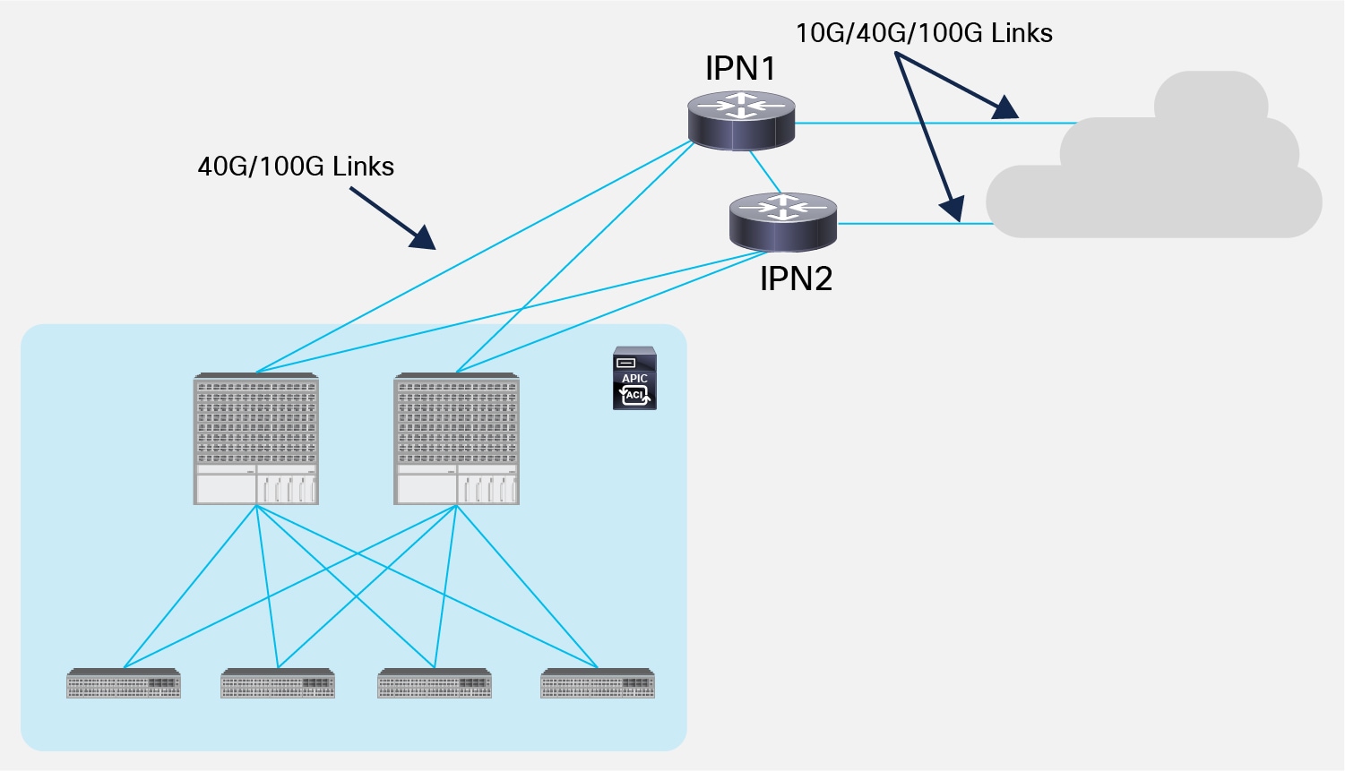
Supported Interface Speed between Spines and IPN Devices
The support of Cisco QSFP to SFP or SFP+ Adapter (QSA) Modules on second-generation spine nodes (for example, modular 9500 switches with second generation EX/FX linecards or 9364C nonmodular spines) allows the use of 10G links for this purpose. Please reference the ACI software release notes to verify support for this connectivity option.
It is also worth noticing that the links connecting the IPN devices to other remote IPN devices (or to a generic Layer 3 network infrastructure) do not need to be 40G/100G. It is however not recommended (although feasible) to use connection speeds less than 10G to avoid traffic congestion across Pods that may affect the communication of APIC nodes deployed in separate Pods.
One of the important properties of Cisco ACI is the capability of bringing up a physical fabric in an automatic and dynamic fashion, requiring only minimal interactions from the network administrator. This is a huge leap when compared to the “box-by-box” approach characterizing traditional network deployments.
The use of a common APIC Controller cluster allows to offer similar capabilities to an ACI Multi-Pod deployment. The end goal is adding remote Pods to the Multi-Pod fabric with minimal user intervention, as shown in Figure 20 below.
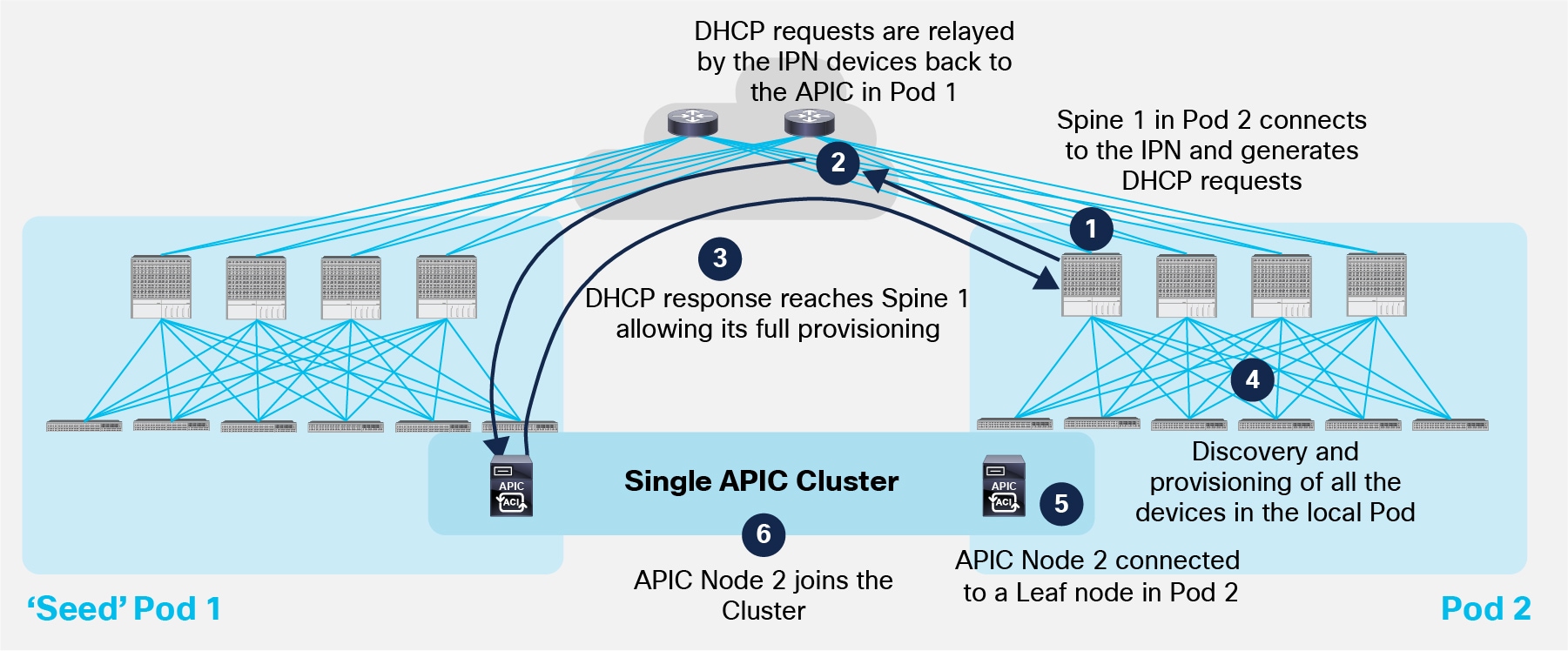
Pod Auto-Provisioning Process
Few initial assumptions before describing the step-by-step procedure required for having a second Pod joining the Multi-Pod fabric:
● The first Pod (also known as ‘Seed’ Pod) has already been set up following the traditional ACI fabric bring-up procedure.
Note: For more information on how to bring up an ACI fabric from scratch please refer to the session available at the link below:
https://www.ciscolive.com/online/connect/search.ww#loadSearch-searchPhrase=paggen&searchType=session&tc=0&sortBy=&p=&i(10017)=20991.
● The ‘Seed’ Pod and the second Pod are physically connected to the IPN devices.
● The IPN devices are properly configured with IP addresses on the interfaces facing the spines and the OSPF routing protocol is enabled (in addition to the MTU, DHCP-Relay and PIM Bidir required configuration). This is a one-time day-0 manual configuration required outside the ACI specific configuration performed on APIC.
As a result of the above assumptions, the IPN devices are peering OSPF with the spines in Pod1 and exchange TEP pool information as discussed in the previous “IPN Control Plane” section. The following sequence of steps allows Pod2 to join the Multi-Pod fabric.
1. The first spine in Pod2 boots up and starts sending DHCP requests out of every connected interface. This implies that the DHCP request is also sent toward the IPN devices.
2. The IPN device receiving the DHCP request has been configured to relay that message to the APIC node(s) deployed in Pod1. Note that the spine’s serial number is added as a TLV of the DHCP request sent at the step above, so the receiving APIC can add this information to its Fabric Membership table.
3. Once a user explicitly imports onto the APIC Fabric Membership table the discovered spine, the APIC replies back with an IP address to be assigned to the spine’s interfaces facing the IPN. Also, the APIC provides information about a bootstrap file (and the TFTP server where to retrieve it (which is the APIC itself) that contains the required spine configuration to set up its VTEP interfaces and OSPF/MP-BGP adjacencies.
Note: In this case the APIC functions also as TFTP server.
4. The spine connects to the TFTP server to pull the full configuration.
5. The APIC (TFTP server) replies with the full configuration. At this point, the spine has joined the Multi-Pod fabric and all the policies configured on the APIC controller are pushed to that device.
Important Note: The spine’s joining process described above gets to completion only if at least a leaf node running ACI code is actively connected to that spine. This is usually not a concern, as in real life deployments there is no use for having a remote spine joining the Multi-Pod fabric if there are no active leaf nodes connected to it.
6. The other spine and leaf nodes in Pod2 would now go through the usual process used to join an ACI Fabric. At the end of this process, all the devices part of Pod2 are up and running and the Pod fully joined the Multi-Pod fabric.
7. It is now possible to connect an APIC node to the Pod. After running its initial boot setup, the APIC node will be able to join the cluster with the node(s) already connected in Pod1. This step is optional as a Pod could join and be part of the Multi-Pod fabric even without having an APIC node locally connected. It is also worth noticing that all the APIC nodes get an IP address from the TEP Pool associated to the ‘seed’ Pod (for example the 10.1.0.0/16 IP subnet). This means that specific host routing information for those IP addresses must be exchanged through the IPN network to allow reachability between APIC nodes deployed across different Pods.
APIC Cluster Deployment Considerations
The ACI Multi-Pod fabric brings some interesting considerations for what concerns the deployment of the APIC controller cluster managing the solutions. In order to understand better the implications of such model, it is useful to quickly review how the APIC cluster works in the regular single Pod scenario.
As shown in Figure 21, a concept known as data sharding is supported for data stored in the APIC in order to increase the scalability and resiliency of the deployment.
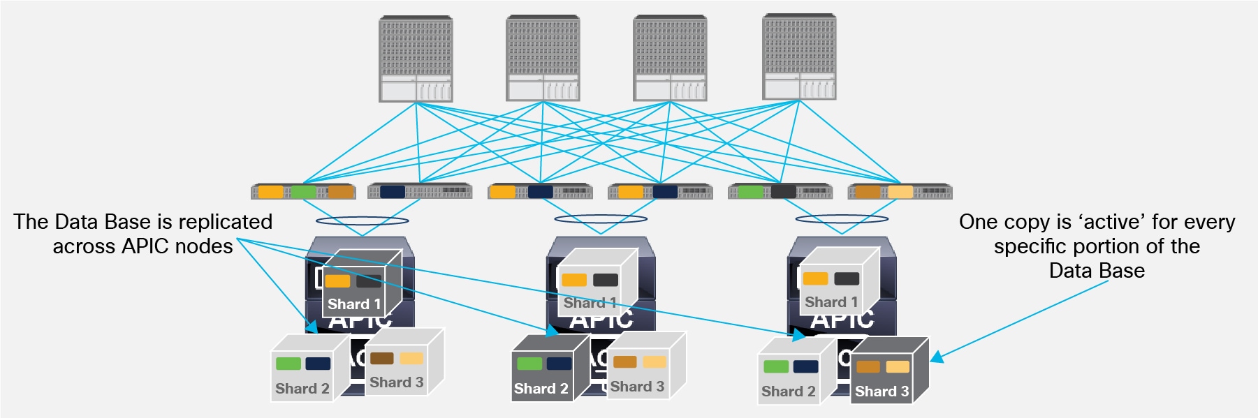
Data Sharding across APIC Nodes
The basic idea behind sharding is that the data repository is split into several database units, known as ‘shards’. Data is placed in a shard, and that shard is then replicated three times, with each copy assigned to a specific APIC appliance. The distribution of shards across a cluster of three and five nodes is shown in Figure 22 below.
Note: To simplify the discussion we can consider the example where all the configuration associated to a given Tenant is contained in a ‘shard’.
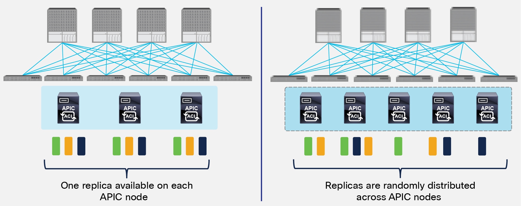
Replicas Distribution across APIC Nodes
In the 3 nodes APIC cluster deployment scenario, one replica for each shard is always available on every APIC node, but this is not the case when deploying a five nodes cluster. This behavior implies that increasing the number of APIC nodes from 3 to 5 does not improve the overall resiliency of the cluster, but only allows supporting a higher number of leaf nodes. In order to better understand this, let’s consider what happens if two APIC nodes fail at the same time.
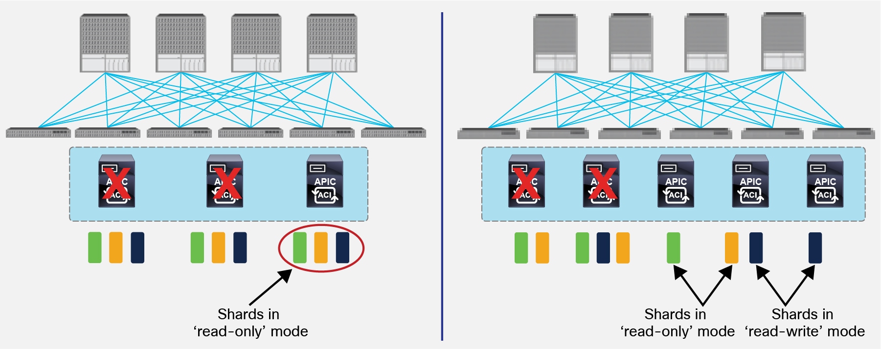
APIC Nodes Failure Scenario
As shown on the left of the figure above, the third APIC node still has a copy of all the shards. However, since it does not have the quorum anymore (it is the only surviving node of a cluster of 3), all the shards are in ‘read-only’ mode. This means that when connecting to the remaining APIC node, no configuration changes can be applied although the node can continue to serve read requests.
On the right, the same dual nodes failure scenario is displayed when deploying a 5 nodes cluster. In this case, some shards on the remaining APIC nodes will be in ‘read-only mode’ (i.e. shards green and orange in this example), whereas other will be in full ‘read-write’ mode (the blue shard). This implies that connecting to one of the three remaining APIC nodes would lead to a non deterministic behavior across shards, as configuration can be changed for the blue shard but not for the green-orange ones.
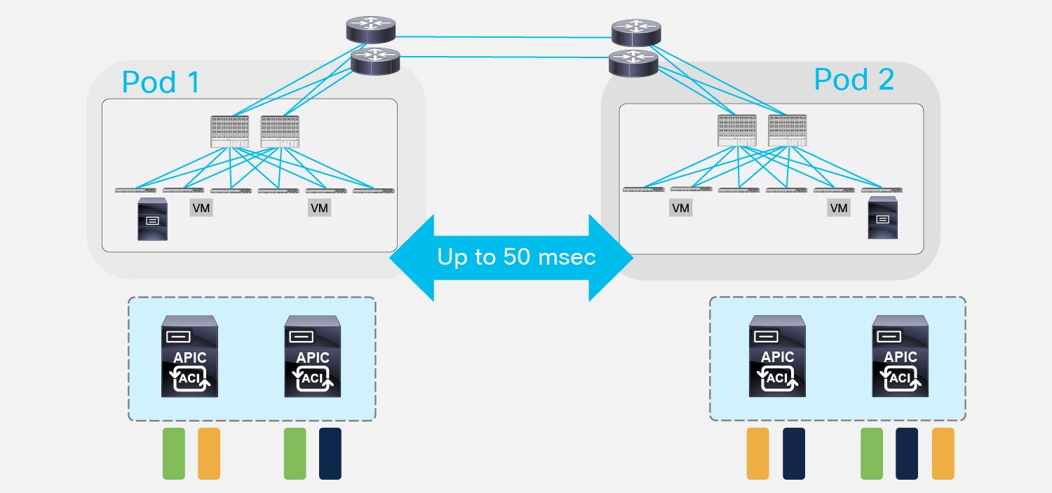
Let’s now apply the considerations above to the specific Multi-Pod scenario where the APIC nodes are usually deployed in separate Pods. The scenario that requires specific considerations is the one where two Pods are part of the Multi-Pod fabric and represent geographically separated DC sites. In this case, two main failure scenarios should be considered:
● A ‘split-brain’ case where the connectivity between the Pods is interrupted (Figure 24).
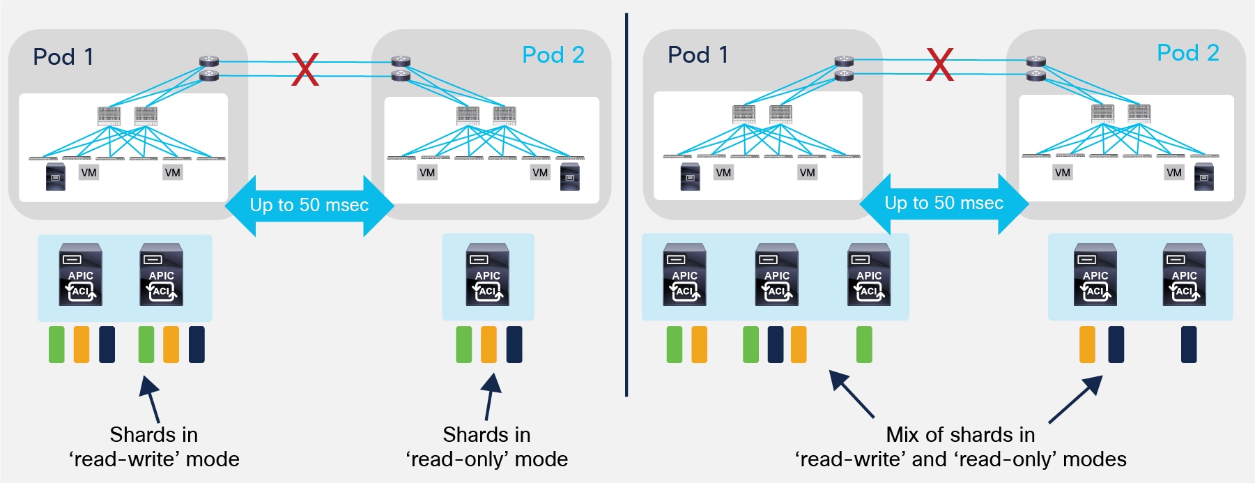
Split-Brain Failure Scenario
In a 3-node cluster scenario, this implies that the shards on the APIC nodes in Pod1 would remain in full ‘read-write’ mode, allowing a user connected there to make configuration changes. The shards in Pod2 are instead in ‘read-only’ mode. For the 5 nodes cluster, the same inconsistent behavior previously described (some shards are in read-write mode, some in read-only mode) would be experienced by a user connecting to the APIC nodes in Pod1 or Pod2.
However, once the connectivity issues are solved and the two Pods regain full connectivity, the APIC cluster would come back together and any change made to the shards in majority mode would be applied also to the rejoining APIC nodes.
● The second failure scenario is instead the one where an entire site goes down because of a disaster (flood, fire, earthquake, etc.). In this case, there is a significant behavioral difference between a 3 or 5 nodes APIC cluster stretched across Pods.
In a 3 nodes APIC cluster deployment, the hard failure of Pod1 causes all the shards on the APIC node in Pod2 to go in ‘read-only’ mode, similarly to what previously described on the left scenario in Figure 23. In this case it is possible (and recommended) to deploy a standby APIC node in Pod2, so to be able to promote it to active once Pod1 fails. This ensures the re-establishment of the quorum for the APIC controller (two nodes out of three would be clustered again).
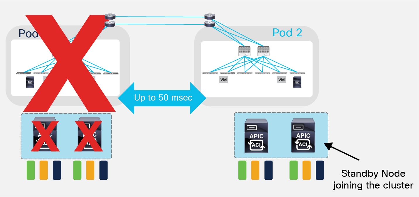
Standby APIC Node Joining the Cluster
The specific procedure required to bring up the standby node and have it joining the cluster is identical to what described for the ACI stretched Fabric design option at the link below (same applies to the procedure to be followed to eventually recover Pod1): https://www.cisco.com/c/en/us/td/docs/switches/datacenter/aci/apic/sw/kb/b_kb-aci-stretched-fabric.html#concept_524263C54D8749F2AD248FAEBA7DAD78.
It is important to reiterate the point that the standby node should be activated only when Pod1 is affected by a major downtime event. For temporarily loss of connectivity between Pods (for example due to long distance link failures when deploying Pods over geographical distance), it is better to rely on the quorum behavior of the APIC cluster. The site with APIC nodes quorum would continue to function without problem, whereas the site with the APIC node in minority would go in read only mode. Once the inter-Pod connection is resumed, the APIC database gets synchronized and all functions fully restart in both Pods.
In a 5 nodes APIC cluster deployment, the hard failure of the Pod with 3 controllers would leave only two nodes connected to Pod2, as shown in Figure 26.
Similar considerations made for the 3 nodes scenario can be applied also here and the deployment of a standby APIC node in Pod2 would allow recreating the quorum for the replicas of the shards available in Pod2. However, the main difference is that this failure scenario may lead to the loss of information for the shards that were replicated across the 3 failed nodes in Pod1 (like the green ones in the example below).
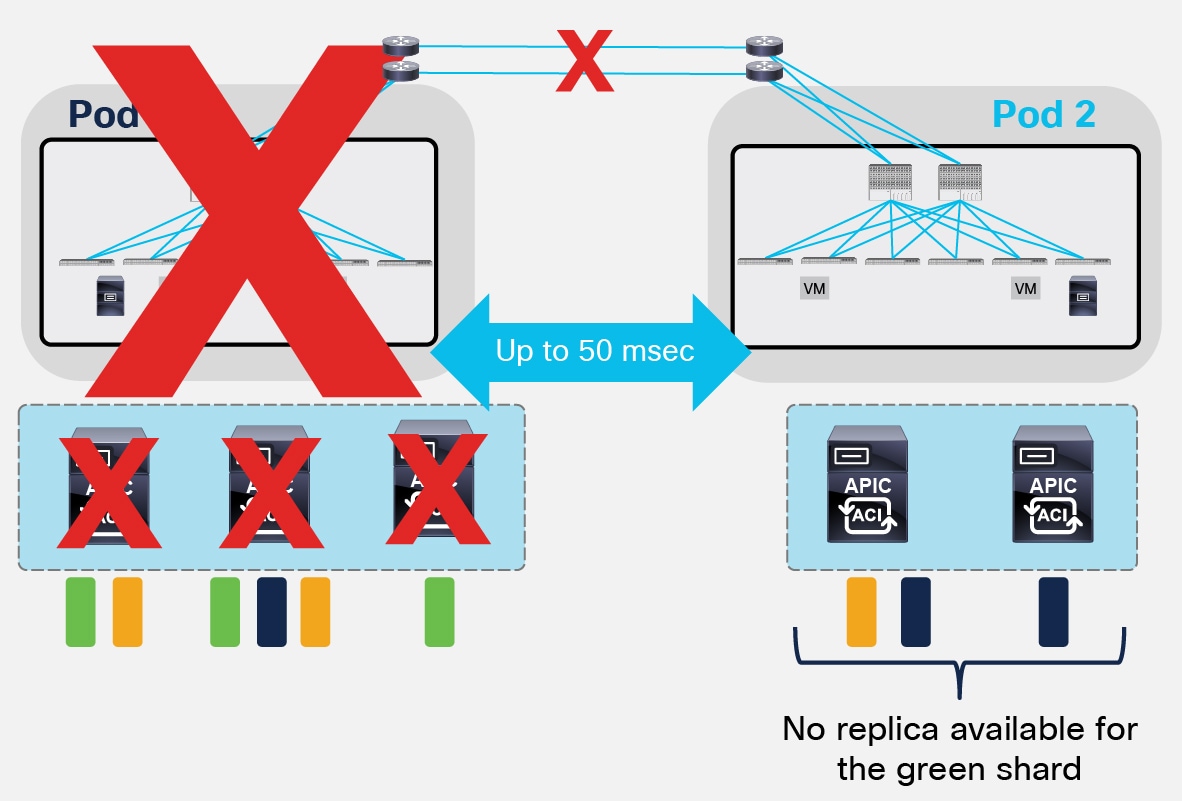
Pod Failure Scenario with a 5 Nodes APIC Cluster
A specific “Fabric Recovery procedure” can be offered starting from ACI 2.2 release to recover the lost shard information from a previously taken snapshot. It is mandatory to contact Cisco TAC or Advanced Services for assistance in performing such procedure.
It is important to notice how this procedure is currently an ‘all or nothing’ implementation: the full APIC cluster and fabric state is restored at time t1 based on the info of the snapshot taken at time t0 and this applies also to the shards whose information was still available in Pod2 (i.e. the orange and blue shards in previous Figure 26). As a consequence, configuration changes (add/delete) for all the shards are lost for the [t0, t1] window, together with statistics, historical fault records and audit-records. Active faults are instead evaluated again once the APIC cluster is reactivated after the completion of the “Fabric Recovery” procedure.
An alternative approach could be to split the 5 nodes APIC cluster between 4 APIC nodes in Pod1 and 1 node in Pod2. This would not protect against the loss of information from some shards after the hard failure of Pod1 (and the consequent need to execute a “Fabric Recovery” procedure); however, it would allow keeping all of the shards in full read-write mode in Pod1 when the two Pods get isolated or after a hard failure of Pod2.
In order to minimize this risk of losing all the three replicas for a shard, the recommendation is to avoid deploying more than two APIC nodes in the same Pod. Starting from ACI software release 4.0(1), it is possible to deploy a 4 nodes APIC cluster to support up to 200 leaf nodes across the two Pods. This deployment model is shown in Figure 27 below.
Multi-Pod Deployment with 4 Active APIC Nodes
The considerations in a split-brain scenario are the same already made for the 5-nodes cluster use case: some shards would be in read-write state in Pod1, some other shards would be in read-write state in Pod2. Once again, this would allow making changes to those shards by connecting to one of the APIC nodes deployed in Pod1 or Pod2, and those changes will then be redistributed across all 4 nodes of the cluster once connectivity between Pods is re-established.
The hard failure of a Pod will instead cause, at worst, the loss of two replicas for the shards, which allows rebuilding a majority state by bringing up a standby APIC node in the remaining Pod (similarly to how discussed for the 3 APIC nodes deployment model).
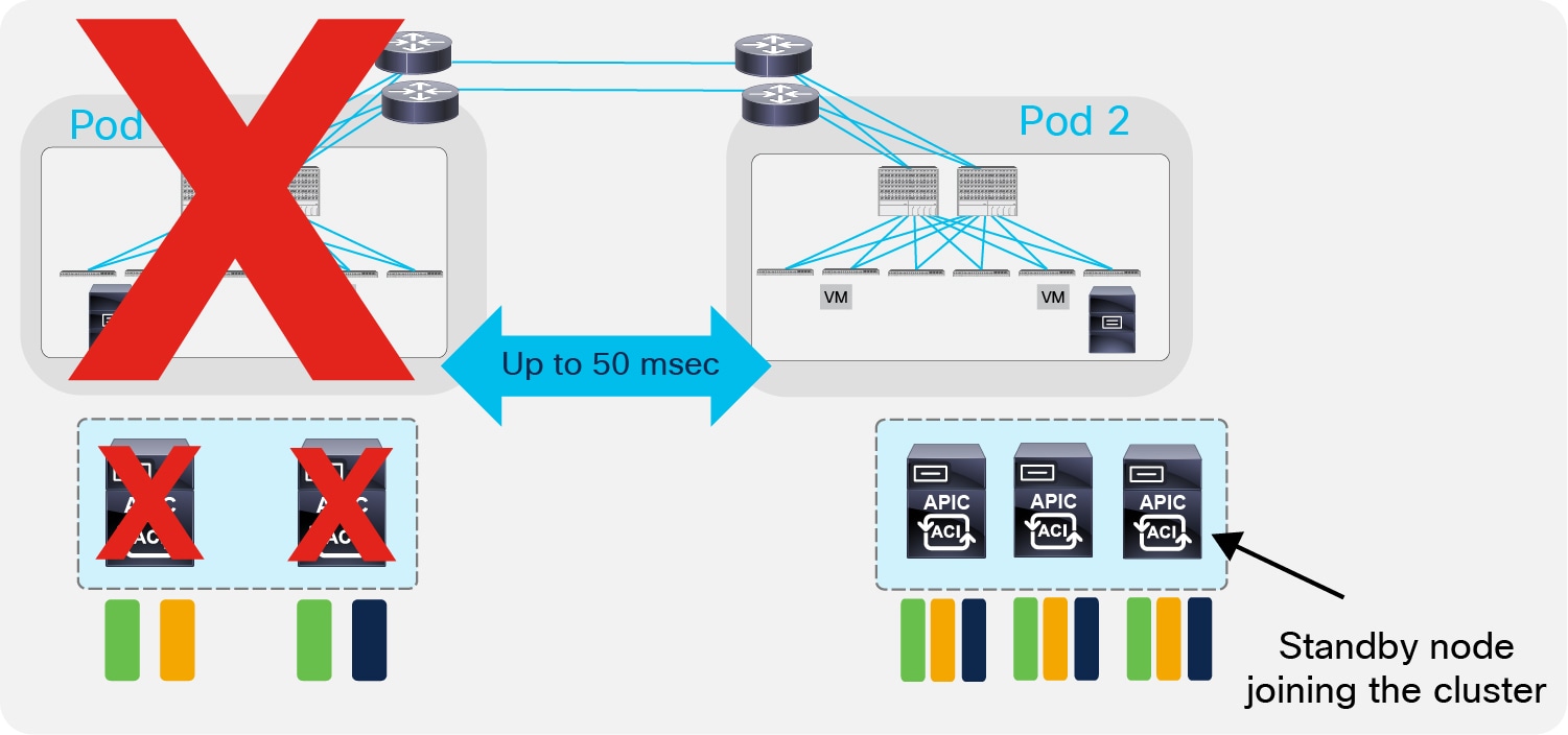
Re-establishment of the Majority State by Activating a Standby APIC Node in Pod2
Based on the above considerations the following recommendations can be made for deploying a two sites Multi-Pod fabric:
1. When possible, deploy a 3 nodes APIC cluster with 2 nodes in Pod1 and one node in Pod2. Add a backup APIC node in Pod2 to handle the full site failure scenario.
2. If more than 80 but fewer than 200 leaf nodes are required across the two Pods, starting from ACI release 4.0(1) the recommendation is to deploy an APIC cluster with 4 active nodes. As mentioned above, a standby APIC could (and should) be deployed inside each Pod for account for the hard failure of one of the Pods.
3. If the scalability requirements force the deployment of a 5 nodes cluster (for example, more than 200 leaf nodes are deployed across the two Pods), whenever possible follow the guidelines depicted in Figure 29 below:
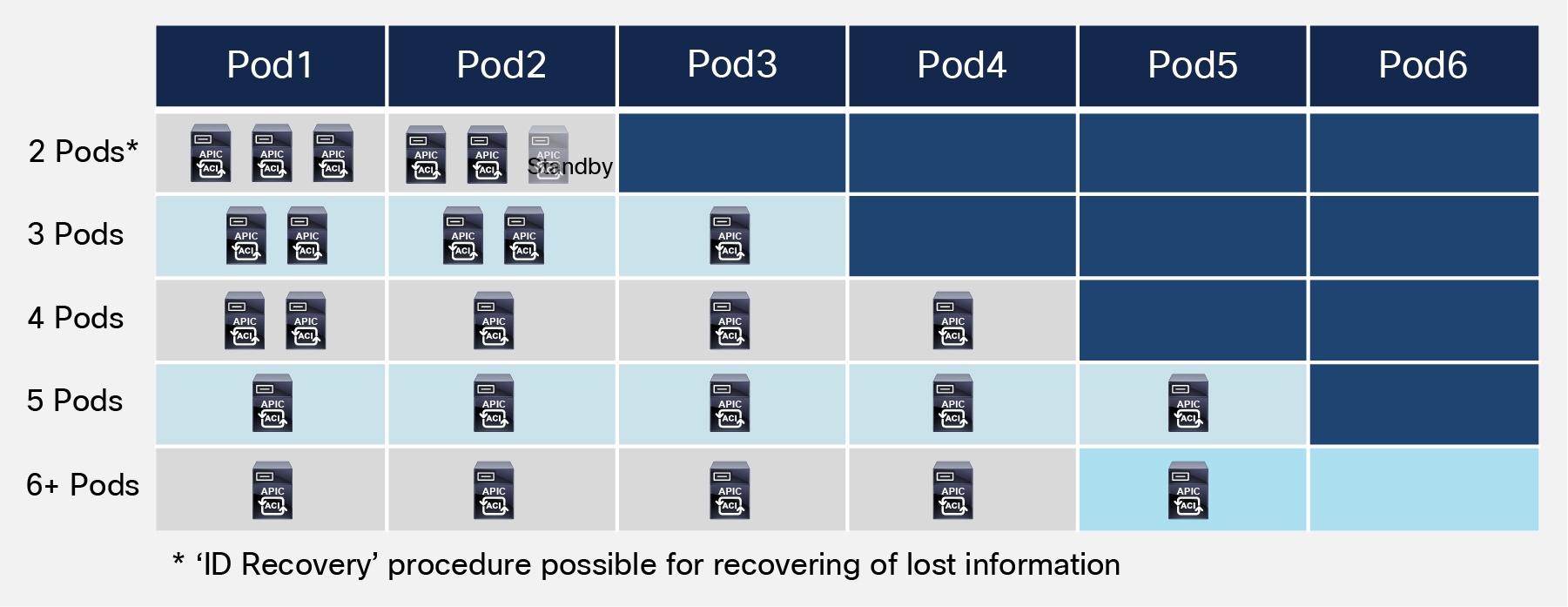
Deployment Guidance for a 5 Nodes APIC Cluster
Two things can be immediately noticed when looking at the table above: first, as previously mentioned, the basic rule of thumb is to avoid deploying 3 APIC nodes in the same Pod, to prevent the potential loss of shards information previously discussed. This recommendation can be followed when deploying 3 or more Pods.
Second, a Pod can be part of the Multi-Pod fabric even without having a locally connected APIC cluster. This would be the case when deploying 6 (or more) Pods leveraging a 5 nodes APIC cluster or when deploying 4 (or more) Pods with a 3 nodes APIC cluster.
Note: Similar considerations apply to the scenario where more than 300 leaf nodes must be supported across Pods, which requires deploying a 7 APIC nodes controller cluster.
Reducing the Impact of Configuration Errors with Configuration Zones
The deployment of a single APIC controller cluster managing all the Pods connected to the same ACI Multi-Pod fabric greatly simplifies the operational aspects of the fabric (providing a single point of management and policy definition).
As a consequence, and similarly to a single Pod ACI deployment, it is possible to make changes that apply to a very large number of leafs and ports, even belonging to separate Pods. While this is one of the great benefit of using ACI because it makes possible to manage a very large infrastructure with minimum configuration burden, it may also raises concerns that a specific configuration mistake that involves many ports may have an impact across all the deployed Pods.
The first solution built in the system to help reducing the chances of making such mistakes is the provision of a button next to each policy configuration that is called “Show Usage”. This allows providing the system and infrastructure administrator with the information of which elements are affected by the specific configuration change he/she is going to make.
In addition to this, a new functionality has been introduced on the APIC controller to limit the spreading of infrastructure configuration changes only to a subset of the leaf nodes deployed in the fabric. This functionality calls for the creation of “Configuration Zones”, where each zone includes a specific subset of leaf nodes connected to the ACI fabric.
Using Configuration Zones lets you test the configuration changes on that subset of leafs and servers before applying them to the entire fabric. Configuration zoning is only applied to changes made at the infrastructure level (i.e. applied to policies in the “Infra” Tenant). This is because a mistake in such configuration would likely affect all the other Tenants deployed on the fabric.
The concept of configuration zone applies very nicely to an ACI Multi-Pod deployment, where each Pod could be deployed as a separate zone (the APIC GUI allows you to directly perform this mapping between an entire Pod and a zone).
Each zone can be in one of these “deployment” modes:
● Disabled: Any update to a node part of a disabled zone will be postponed till zone deployment mode is changed or the node is removed from the zone.
● Enabled: Any update to a node part of an enabled zone will be immediately sent. This is the default behavior. A node not part of any zone is equivalent to a node part of a zone set to enabled.
Changes to the infrastructure policies are immediately applied to nodes that are member of a deployment mode enabled zone. These same changes are queued for the nodes that are member of a zone with deployment mode disabled.
You could then verify that the configurations are working well on the nodes of the zone deployment mode enabled, and then change the deployment mode to “triggered” for the zones that are in deployment mode disabled in order for these changes to be applied on the leafs in this other zone.
Multi-Pod “Overlay” Control and Data Planes
The ACI Multi-Pod fabric leverages different control and data plane functionalities for connecting endpoints deployed across different Pods.
Inter-Pods MP-BGP Control Plane
In a single ACI fabric, information about all the endpoints connected to the leaf nodes is stored in the Council of Oracle Protocol (COOP) database available in the spine nodes. Every time an endpoint is discovered as locally connected to a given leaf node, the leaf originates a COOP control plane message to communicate the endpoint information (IPv4/IPv6 and MAC addresses) to the spine nodes. The COOP protocol is also leveraged by the spines to synchronize this information between them.
The same information about discovered endpoints must be maintained between spine nodes part of separate Pods, since functionally the Multi-Pod fabric must behave like a single fabric. An independent instance of the COOP protocol is running between the leaf and spine nodes in each Pod; hence the MP-BGP control plane between spines is introduced for synchronizing reachability information across Pods. This functionality is shown in Figure 30 below.
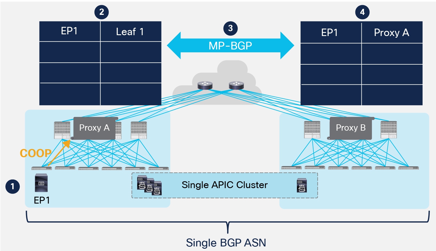
MP-BGP Control Plane across Pods
1. An endpoint EP1 connects to Leaf 1 in Pod1. The leaf discovers the endpoint and sends a COOP control plane message to the Anycast VTEP address representing all the local spines.
2. The receiving spine adds the endpoint information to the COOP database and synchronizes the information to all the other local spines. EP1 is associated to the VTEP address identifying the local leaf nodes where it is connected.
3. Since this is the first time the endpoint is added to the local COOP database, an MP-BGP update is sent to the remote spine nodes to communicate the endpoint information.
Note: As an implementation details, it is worth noticing that MAC/IP address information for the endpoints are exchanged between spines in different Pods leveraging the MP-BGP EVPN address-family (using Type-2 EVPN advertisements), whereas IPv4/IPv6 prefixes (as for example the ones relative to destination external to the ACI fabric) are exchanged via VPNv4 address-family.
4. The receiving spine node adds the information to the COOP database and synchronizes it to all the other local spine nodes. EP1 is now associated to an Anycast VTEP address (“Proxy A”) available on all the spine nodes deployed in Pod1. This behavior provides a robust control plane isolation function across Pods, as there is no requirement to send new control plane updates toward Pod2 even if EP1 moves many times across leaf nodes part of Pod1, since the entry would continue to point to the “Proxy A” next-hop address.
As shown in Figure 30, all the Pods are part of the same BGP Autonomous System. As a consequence, the peering between spine nodes can be performed in two ways:
● Establishing a full mesh of MP-iBGP sessions between all the spines (local and remote). This is the default behavior and is shown in Figure 31.
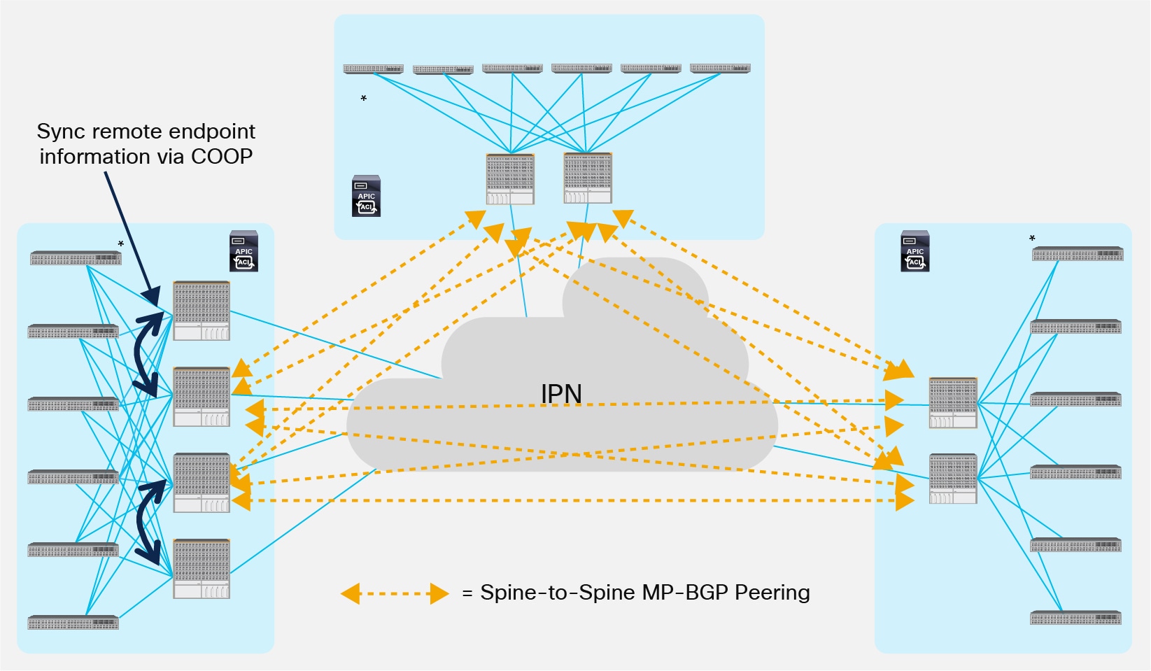
Full Mesh of MP-iBGP Sessions across Pods
Note: It is not recommended to establish inter-Pod MP-BGP EVPN peerings on more than one pair of spine devices in each Pod, independently from the total number of spines deployed in the Pods. This is to contain the overall number of inter-Pod adjacencies established across Pods. The other spines deployed in the Pod (spines 1 and 4 in the example in Figure 31, above) can still be leveraged for inter-Pod data-plane communication even if they don’t establish EVPN peerings with the spines in the remote Pods as they receive remote endpoint information through COOP from the other local spines EVPN enabled. A specific “External Control Peering” flag is available in the logical node profile for each spine part of the “infra” L3Out to control the establishment of inter-Pods EVPN adjacencies. In the example in figure above, the flag would need to be checked in Pod1 for spines 2 and 3 and un-checked for spines 1 and 4. In this scenario, COOP is used internally to a Pod to sync remote endpoint information between the spines that have BGP enabled and the ones that do not establish EVPN peerings with the remote Pods.
● Defining Route-Reflector devices in each Pod so that the spine nodes only peer with the remote RR nodes and a full mesh of MP-iBGP session is then established between the RRs. Those External RR nodes (Ext-RRs) serve a different function from the Internal RR nodes (Int-RRs) that are always deployed for distributing to all of the leaf nodes that are part of the same Pod external IPv4/IPv6 prefixes learned on the L3Out logical connections (for more information, refer to the “Connectivity to the External L3 Domain” section).
The best-practice recommendations for the deployment of Ext-RR nodes, due to specific internal implementation, are the followings:
● Ensure that any spine node that is not configured as Ext-RR is always peering with at least one Ext-RR node. Since spines do not establish intra-Pod EVPN adjacencies, this implies that a spine that is not configured as an Ext-RR node should always peer with two remote Ext-RRs (in order to continue to function if a remote Ext-RR node should fail). This means it makes little sense to configure Ext-RRs for a 2 Pods deployment, since it does not provide any meaningful savings in terms of overall EVPN adjacencies that need to be established across the Pods.
● For a 3 Pods (or more) Multi-Pod fabric deployment, define one Ext-RR node in the first 3 Pods only (3 Ext-RR nodes in total), as shown in Figure 32.
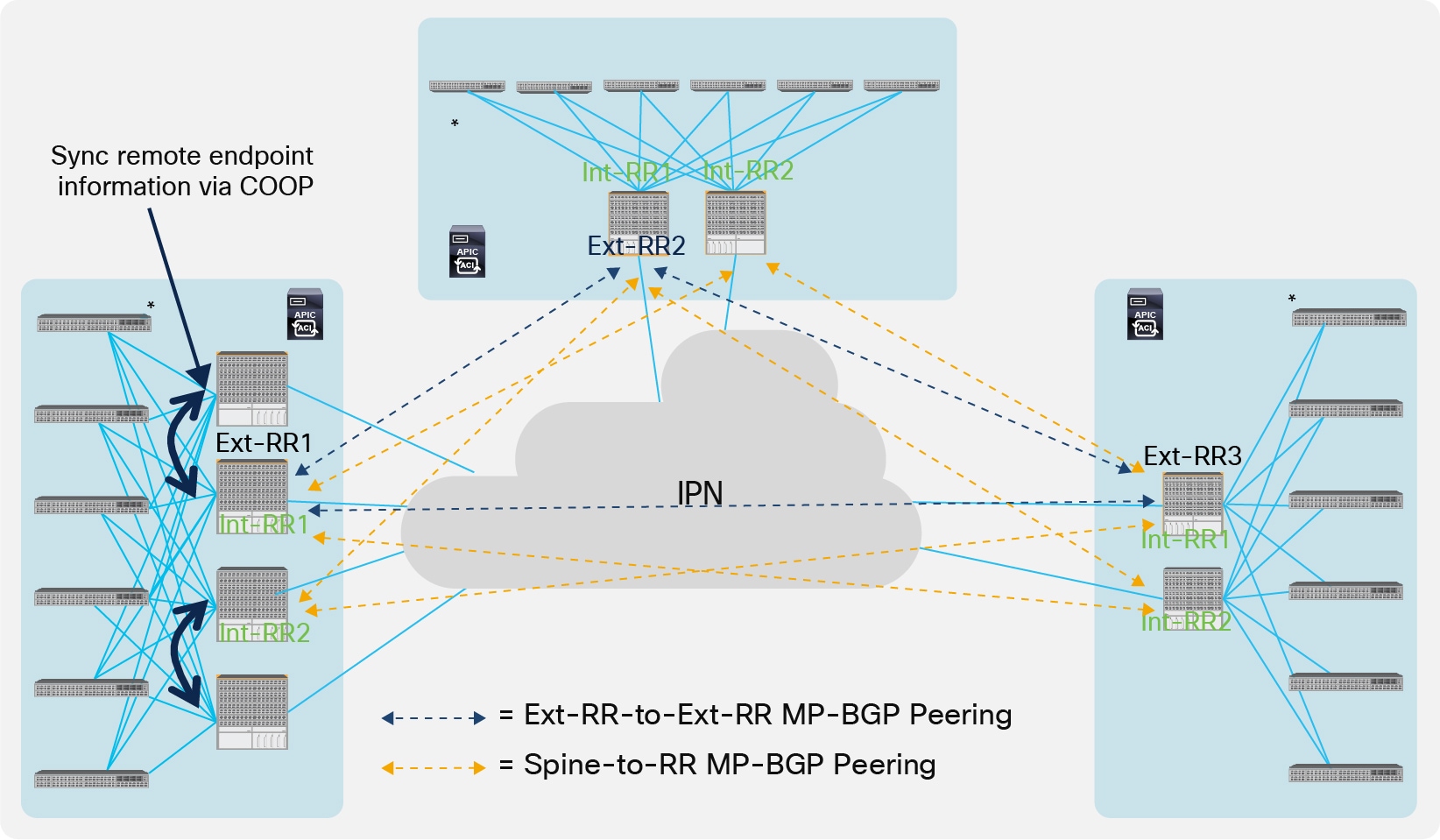
Defining a Route-Reflector per Pod
● For a Multi-Pod deployment with 4 Pods (or more), it is recommended to deploy Ext-RRs and not to create full-mesh peerings between the spines. A maximum of 4 Ext-RRs are supported in a Multi-Pod fabric. Depending on the geographical distribution of the Pods, the Ext-RRs should be distributed across Pods so that under any failure scenario there are always (at least) two Pods with Ext-RRs reachable (i.e. the other spines deployed in the same Pod with an Ext-RR should always be able to peer with at least one Ext-RR in a remote Pod).
● Deploy the Ext-RR node function on the same spine already used as the Int-RR node for replicating external prefixes to the leaf nodes part of the local Pod.
The deployment of the ACI Multi-Pod fabric allows to seamlessly achieve Layer 2 and Layer 3 communication between endpoints connected to separate Pods. The mechanism to achieve such communication is similar in those two cases and will be described in the rest of this section. The assumption is that IP communication is required, either intra-subnet or inter-subnet (for non IP communication the behavior is the one already described in the “IPN Multicast Support” section).
In order to establish IP connectivity between endpoints connected to separate Pods, the first requirement is to be able to complete an ARP exchange. A slightly different mechanism is implemented depending on the specific Bridge Domain configuration, specifically with regard with the enablement or not of ARP flooding.
Figure 33 shows the scenario where ARP flooding is enabled on the Bridge Domain where both EP1 and EP2 belong. The assumption is that both EP1 and EP2 haven’t been discovered yet (they are both considered ‘silent hosts’), since this is the most complex scenario.
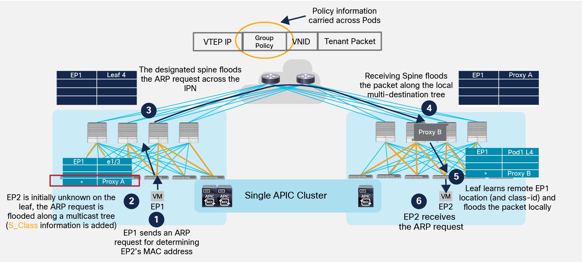
ARP Request with ARP Flooding Enabled
1. EP1 generates an ARP request to determine EP2’s MAC address (assuming EP1 and EP2 are part of the same IP subnet).
2. The local leaf receives the packet, inspects the payload of the ARP packet and learns EP1 information (as a locally connected endpoint) and knows the ARP request is for EP2’s IP address. Since EP2 has not been discovered yet, the leaf does not find any information about EP2 in its local forwarding tables. As a consequence, since ARP flooding is enabled, the leaf picks the FTAG associated to one of the multi-destination trees used for BUM traffic and encapsulates the packet into a multicast packet (the external destination address is the GIPo associated to the specific BD). While performing the encapsulation, the leaf also adds to the VXLAN header the S_Class information relative to the End Point Group (EPG) that EP1 belongs to.
3. The designated spine sends the encapsulated ARP request across the IPN, still leveraging the same GIPo multicast address as the destination of the VXLAN encapsulated packet. The IPN network must have built a proper state to allow for the replication of the traffic toward all the remote Pods where this specific BD has been deployed.
4. One of the spine nodes in Pod2 receives the packet (this is the specific spine that previously sent toward the IPN an IGMP Join for the multicast group associated to the BD) and floods it along a local multi-destination tree. Notice also that the spine has learned EP1 information from an MP-BGP update received from the spine in Pod1.
5. The leaf where EP2 is connected receives the flooded ARP request, learns EP1 information (location and class-id) and forwards the packet to all the local interfaces part of the BD.
6. EP2 receives the ARP request and this triggers its reply allowing then the fabric to discover it (i.e. it is not a ‘silent host’ anymore).
Figure 34 highlights the completion of the ARP exchange between EP1 and EP2.
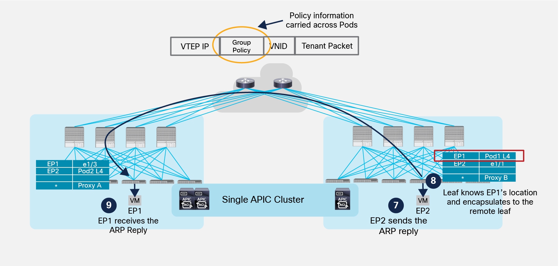
Completion of ARP Exchange
7. EP2 generates a unicast ARP reply destined to EP1 MAC address.
8. The local leaf has now EP1 location information so the frame is VXLAN encapsulated and destined to Leaf 4 in Pod1. At the same time, the local leaf also discovers that EP2 is locally connected and informs the local spine nodes via COOP.
9. The remote leaf node in Pod1 receives the packet, decapsulates it, learns and programs in the local tables EP2 location and class-id information and forwards the packet to the interface where EP1 is connected. EP1 is hence able to receive the ARP reply.
It is worth noticing how ACI was designed to handle the presence of silent hosts even without requiring the flooding of ARP requests inside the Bridge Domain. Without ARP flooding allowed in the Bridge Domain, the leaf nodes are not allowed to flood the frame along the local multi-destination tree, so in order to ensure the ARP request can be delivered to a remote endpoint for allowing its discovery, a process named “ARP Gleaning” has been implemented.
With ARP Gleaning, if the spine does not have information on where the destination of the ARP request is connected, the fabric generates an ARP request originated from the IP address associated to the Bridge Domain. This ARP request is sent out all the leaf nodes edge interfaces part of the Bridge Domain. In the specific Multi-Pod scenario, the ARP Glean request is also sent to the remote Pods across the IPN, as shown in Figure 35 below.
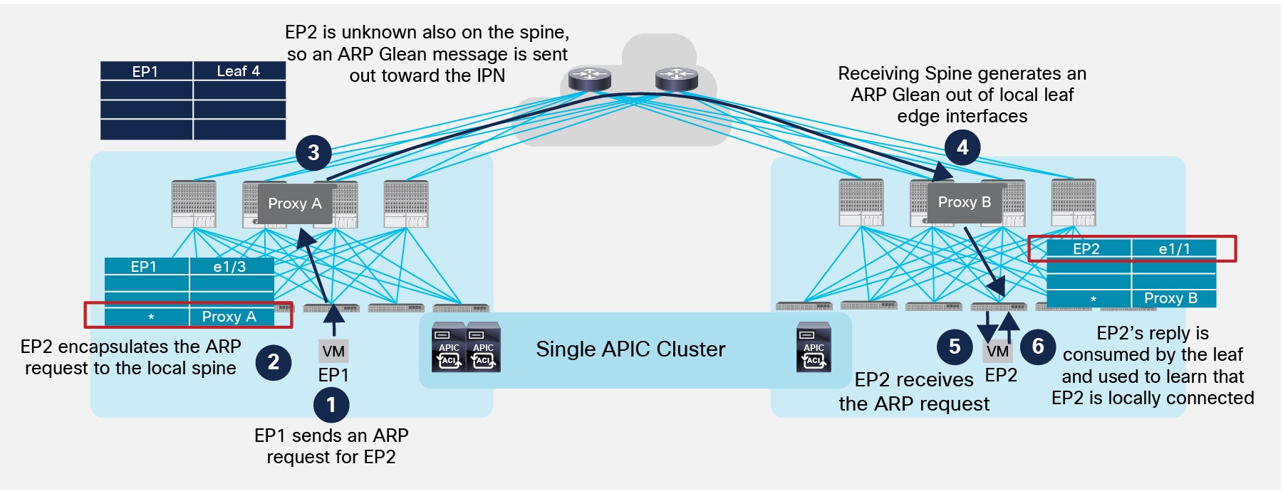
Use of ARP Glean Messages across Pods
1. EP1 generates an ARP request to determine EP2’s MAC address.
2. The local leaf does not have EP2’s information but since ARP flooding is disabled it encapsulates the ARP request toward one of the Proxy Anycast VTEP addresses available on the local spine nodes (no flooding along the local multi-destination tree is allowed).
3. The receiving spine decapsulates the packet and since it does not have EP2 information, an ARP Glean message is sent out all the local leaf edge interfaces part of the same BD and also in the IPN network. The ARP Glean message is a L2 broadcast ARP request sourced from the MAC address associated to the BD. As a consequence, it must be encapsulated into a multicast frame before being sent out toward the IPN. The specific multicast group 239.255.255.240 is used for sourcing ARP Glean messages for all the BDs (instead that the specific GIPo normally used for BUM traffic in a BD).
4. One of the spine nodes in the remote Pod previously sent an IGMP join for the 239.255.255.240 group (since the BD is locally defined), so it receives the packet, performs VXLAN decapsulation and generate an ARP Glean message that is sent to all the leaf nodes inside the Pod, so it reaches also the specific leaf where EP2 is locally connected.
5. The leaf receives the Glean message and forwards it to EP2.
6. EP2 sends the ARP reply, the packet is locally consumed by the leaf (since the destination MAC is the one associated to the SVI of the BD locally defined), which learns EP2 location information.
At this point, the leaf can send a COOP update to the local spines, which then announces the information to the remote spines via MP-BGP. This implies that EP2 is now known also in Pod1 and when EP1 generates another ARP request, the ARP request can be sent across Pods encapsulated in a unicast VXLAN packet destined to the Anycast Proxy-VTEP address identifying the spines in the remote Pod, as shown in Figure 36.
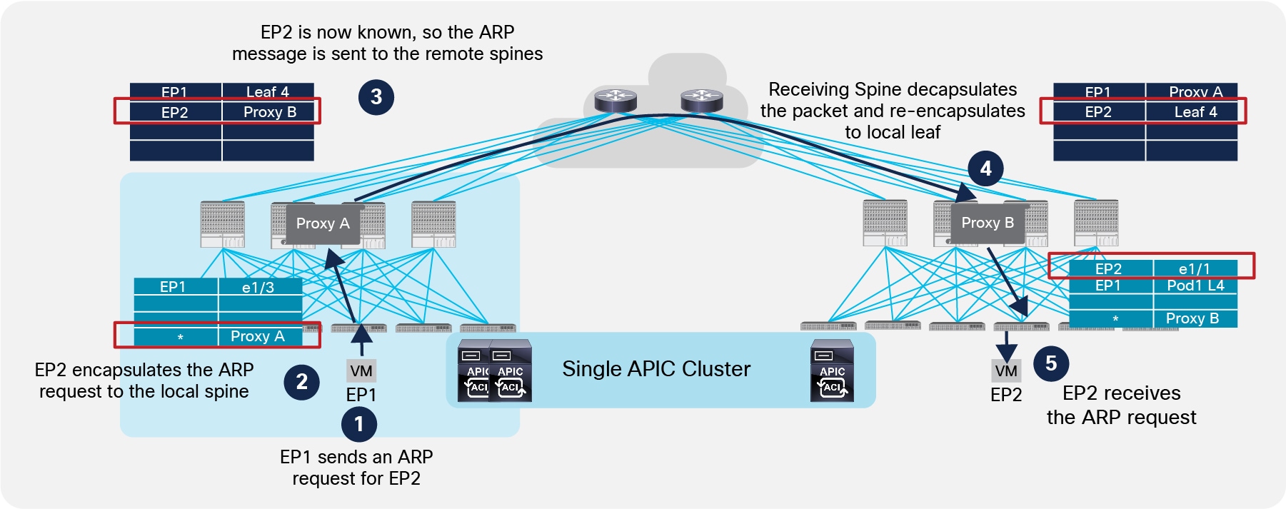
Completion of ARP Exchange with ARP Flooding Disabled
Notice at step 5, the leaf also can learn EP1’s location, so the ARP reply is then sent back from Pod2 to Pod1 following the same steps sequence shown in Figure 34.
Below are a couple of important considerations relative to the ARP Glean functionality:
● The ARP Gleaning mechanism is only possible when an IP address is configured for the Bridge Domain. For this reason, even in cases where the ACI fabric is only used for Layer 2 services (for example when deploying an externally connected default gateway), the recommendation is to configure an IP address in the BD when the goal is to disable ARP flooding (this IP address clearly must be different from the external default gateway used by the endpoints part of the BD).
● As previously mentioned, the destination IP address of the encapsulated ARP Glean frame sent into the IPN is a specific multicast address (239.255.255.240), which is used for performing ARP gleaning for all the defined Bridge Domains. Since this multicast group is normally different from the range used for flooding Bridge Domain’s traffic (each BD by default makes use of a GIPo part of the 225.0.0.0/15 range), it is critical to ensure the IPN network is properly configured to handle this traffic.
Once the ARP exchange is completed, both endpoints EP1 and EP2 are fully discovered and it is hence possible to establish data plane communication.
Data Plane Communication across Pods
Communication between endpoints belonging to separate Pods is achieved with the establishment of end-to-end VXLAN tunnels between the leaf nodes where those endpoints are connected. From a security perspective, the policy enforcement is always applied at the ingress leaf node.
Note: The example above focused on communication between two endpoints that are part of the same IP subnet, but very similar considerations apply when EP1 and EP2 are part of separate IP subnets.
Live Workload Migration Across Pods
As previously clarified, the deployment of an ACI Multi-Pod fabric allows by definition to extend BD connectivity across separate Pods; as a result, this provides flexibility for where to connect endpoints part of a given BD. At the same time, the ACI Multi-Pod fabric supports also live mobility for endpoints between leaf nodes of the same Pod or even across separate Pods. The step-by-step process required to minimize the traffic outage during a workload live migration event is described in the figures below.
Figure 38 shows the initial state, where two endpoints connected to the same Pod are actively communicating with each other.
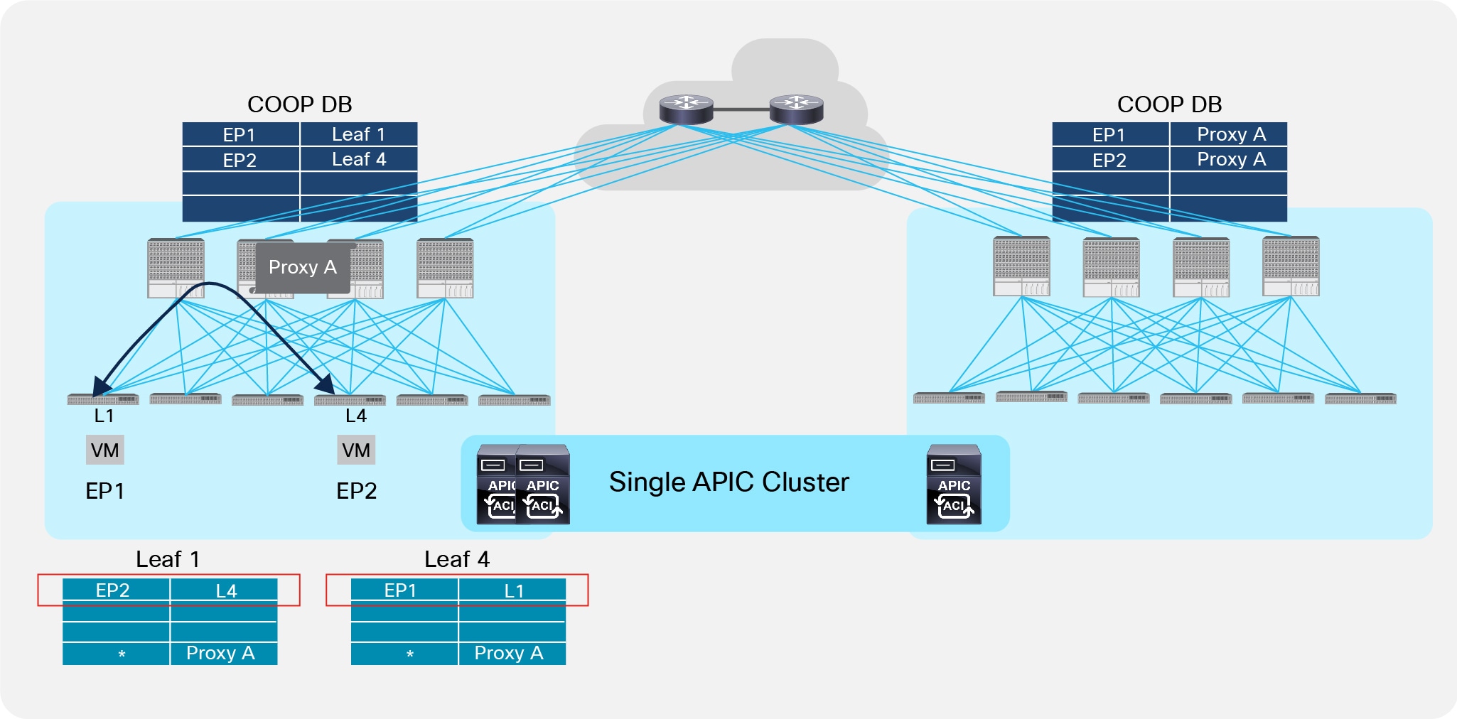
Initial Communication between Endpoints Part of the Same Pod
As shown above, a VXLAN tunnel is established between the two leaf nodes inside the Pod to enable the communication between the endpoints.
Figure 39 shows the sequence of steps required to maintain communication between the endpoints when EP2 is migrated from Pod1 to Pod2.
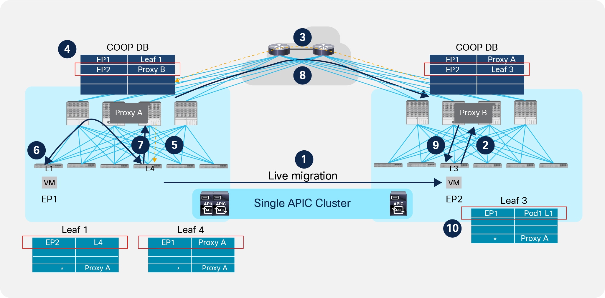
Live Migration across Pods
1. The VM migrates between Pod1 and Pod2.
2. Once the migration is completed, the leaf node in Pod2 discovers EP2 as locally connected and sends a COOP update message to the local spines.
3. The spine node that receive the COOP message updates EP2’s info in the COOP database, replicates the information to the other local spines and sends a MP-BGP EVPN update to the spines in remote Pods.
4. The spines in the remote Pods receive the EVPN update and add the information to the local COOP database that EP2 is now reachable via the Proxy VTEP address identifying the spines in Pod2 (“Proxy B”).
5. The spine sends a control plane message to Leaf 4 as it was the old known location for EP2. Leaf 4 as a consequence installs a bounce entry for EP2 pointing to the local spines Proxy VTEP address.
6. EP1 keeps sending traffic destined to EP2 to the old location (Leaf 4 in Pod1).
7. Leaf 4 has the bounce entry previously described, hence it encapsulates received traffic destined to EP2 toward the local spines.
8. The local spine receiving the packet decapsulates it and performs a lookup in the database. It now has updated information about EP2, so it re-encapsulates traffic to the remote spine nodes.
9. The receiving spine in Pod2 has also updated information about EP2’s location, so it encapsulates traffic to the local Leaf 3 node.
10. Once Leaf 3 receives the packet, it learns EP1’s location (assuming it is the first time EP1 communicates with a locally connected endpoint) and sends the traffic to EP2.
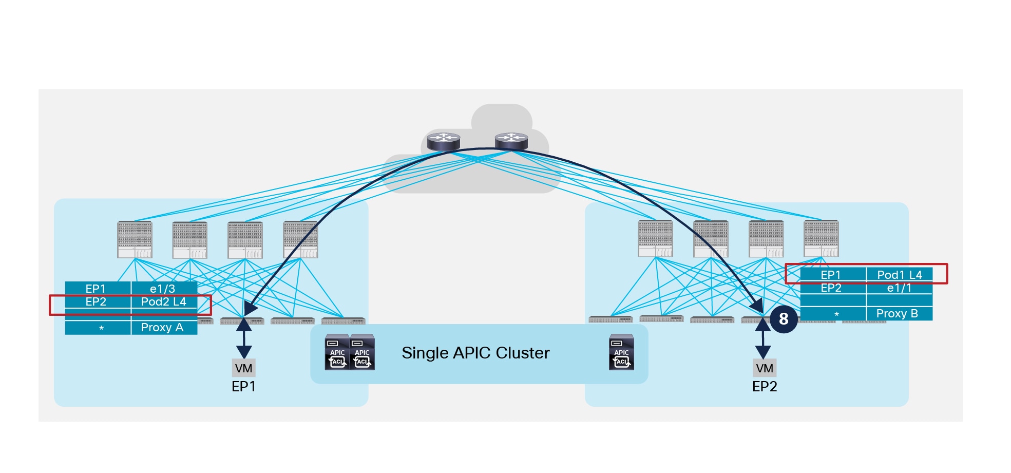
Figure 40 shows the final steps required to establish a direct VXLAN tunnel between the leaf nodes deployed in separate Pods.
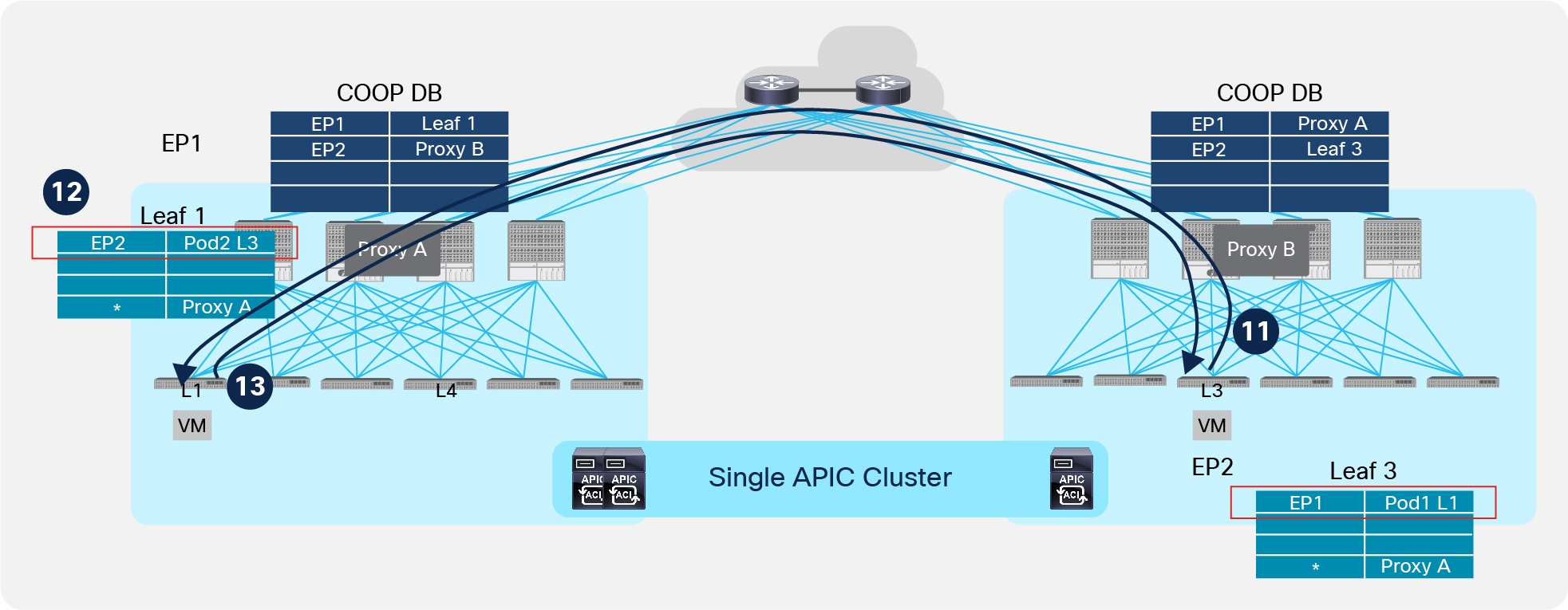
Establishment of End-to-End VXLAN Tunnels across Pods
11. EP2 sends traffic to EP1. Leaf 3 has specific information about EP1’s location, so it encapsulates the traffic directly toward remote Leaf1 in Pod1.
12. When Leaf 1 receives the packet, it updates EP2’s location information to point directly to the remote Leaf 3 in Pod2.
13. Data packets sent from EP1 and destined to EP2 can now be directly encapsulated toward the remote Leaf 3 node.
Connectivity to the External L3 Domain
Connectivity between the ACI fabric and the external routed network domain is normally achieved with the definition of one (or more) Layer 3 connections named L3Outs. An L3Out is a logical connection established between one or more pair of ACI leaf nodes (named Border Leafs) and WAN Edge routers deployed externally to the ACI fabric. Each VRF deployed inside the fabric can leverage those L3Out connections for establishing ‘VRF-Lite’ connectivity with external routers. That way, a separate instance of a routing protocol (or alternatively static routing) can be deployed for each VRF.
Alternatively, if all the BDs (or VRFs) defined inside the ACI fabric must have access to a common external routing domain, it is possible to define a single L3Out connection shared by all those entities and usually defined as part of the “common” tenant.
Note: The L3Out connections are traditionally established from ACI Border Leaf nodes. An alternative approach, named “GOLF,” allows the creation of L3Out connections leveraging the EVPN control plane and the VXLAN data plane between the ACI spines and the external Layer 3 devices. GOLF deployment is not discussed in the context of this paper, for more information please refer to the Cisco Live presentation below: https://www.ciscolive.com/global/on-demand-library/?search=BRKACI-2220#/session/14752114892050019coG.
The routing information learned from the external network domain on the L3Outs connections is redistributed inside the ACI fabric by the Border Leafs. The control plane used for this function is MP-BGP; more specifically, given the multi-tenant nature of the ACI fabric, the VPNv4 address-family is leveraged for sending external routing information to all the deployed leaf nodes, for each defined VRF.
In a traditional single Pod ACI deployment, a pair of spines are designated as MP-BGP VPNv4 Route-Reflectors (RRs), so that all the leaf nodes deployed in the fabric peer with the RRs in order to receive external routing information from the Border Leafs.
Note: For more information about the deployment of L3Out in an ACI fabric please refer to the links below: https://www.cisco.com/c/en/us/solutions/collateral/data-center-virtualization/application-centric-infrastructure/white-paper-c07-732033.html.
L3Outs are also used to achieve external connectivity in ACI Multi-Pod fabric deployments. In a Multi-Pod fabric, a pair of RR nodes are defined in each Pod to perform this RR functionality internally to the Pod they belong to. This role should not therefore be confused with the optional External RR role used to distribute endpoint information across Pods, as previously discussed in the “Inter-Pods MP-BGP Control Plane” section.
Let’s consider the example in Figure 41 below where three Pods are interconnected with each other in a triangle.
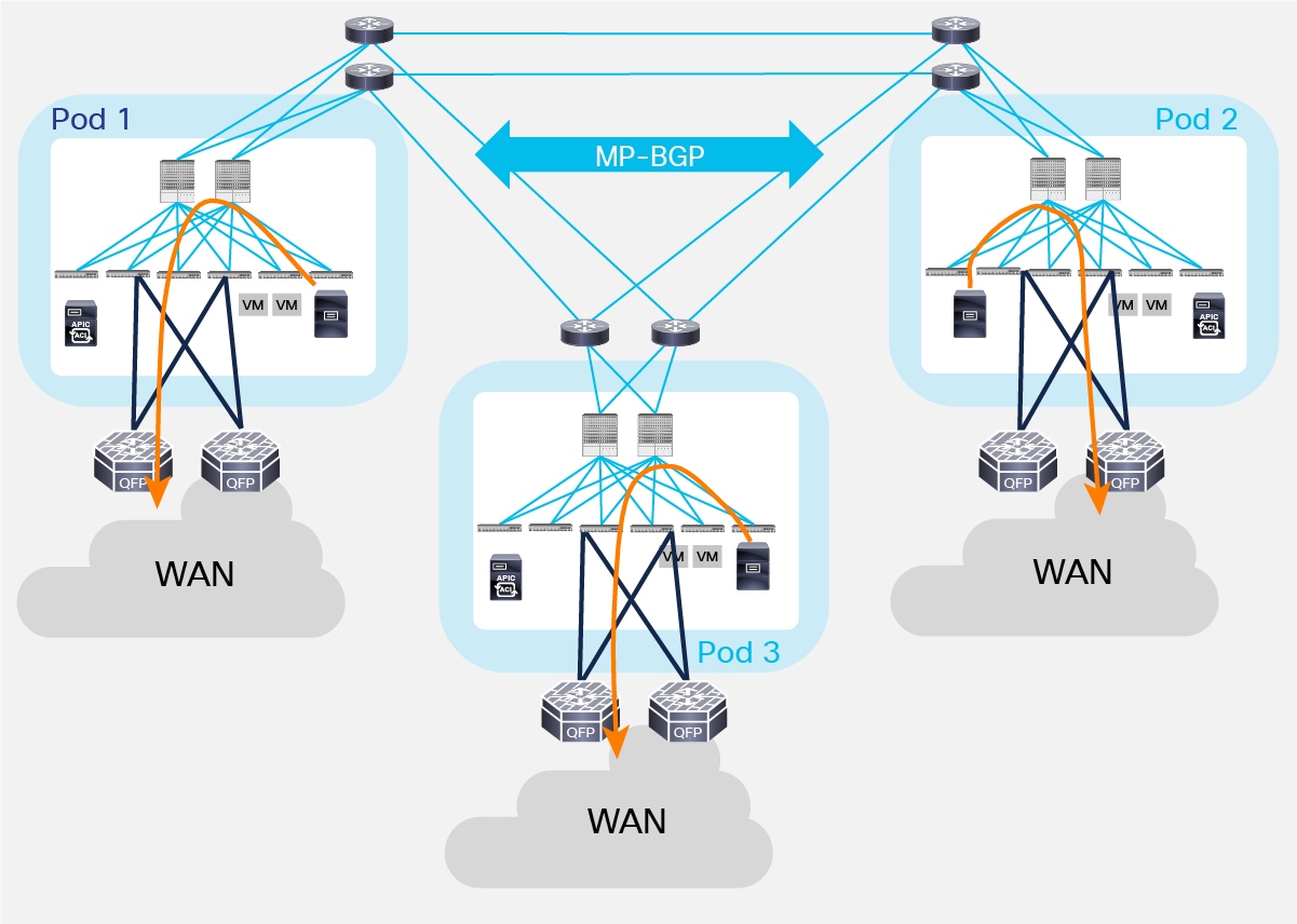
Different L3Outs in Separate Pods
Depending on the distance between the separate Pods, it may be desirable that each Pod leverages its own connection to the external network domain, as shown in Figure 41. This would typically be the case when Pods represent physical data center sites that are geographically separated. This behavior may or may not be the default one, depending on the following considerations:
● If the same external prefix was injected inside the Multi-Pod fabric from each L3Out connection while using OSPF or EIGRP as a control-plane protocol with the external routers, endpoints deployed in a given Pod would always leverage the local L3Out connection to send traffic to external destinations. This is because external prefixes are injected by the border leaf nodes in each Pod into the BGP VPNv4 fabric control plane and from a routing metric perspective, the path toward the local BL nodes is preferred to the one leading to border leaf nodes in remote Pods.
● If the same external prefix was injected inside the Multi-Pod fabric from each L3Out connection while using BGP as the control-plane protocol with the external routers, the specific BL nodes selected for sending outbound traffic would depend on the BGP attributes carried in the updates from the external routers. If those attributes were the same, then the behavior would be identical to the one discussed in the previous bullet point for OPSF and EIGRP peering. If, instead, a prefix received on the L3Out of a specific Pod had a better specific attribute (for example, AS-Path) compared to the same prefixes received on the L3Outs of the other Pods, the first L3Out would become the preferred outbound connection for all the leaf nodes deployed in the Multi-Pod fabric.
In case of failure of both border leaf nodes deployed inside a Pod, or in WAN failure scenarios where external prefixes are not reachable anymore via the local L3Out connection, endpoints can continue to communicate with the external Layer 3 domain leveraging the L3Out connections in remote Pods (the specific L3Out that will be utilized would depend on the consideration made). Figure 42 shows an example where traffic will be load-balanced on a per-flow basis via the L3Out connections available in Pod 2 and Pod 3.
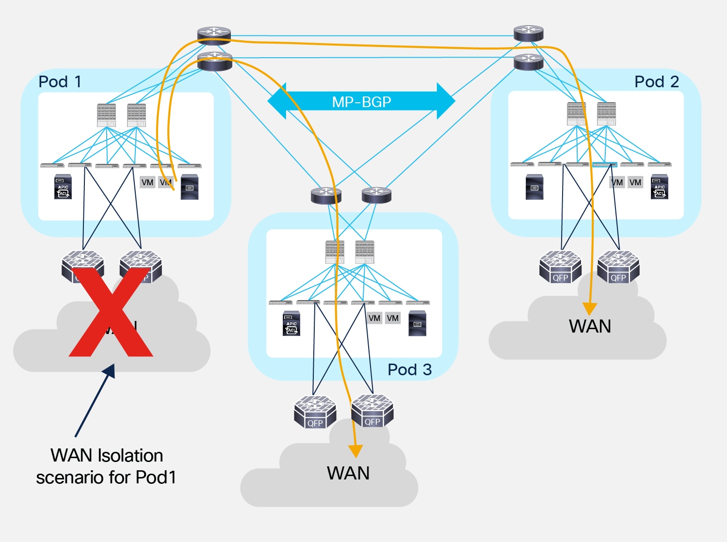
Use of remote L3Out connections for outbound traffic
The load-balancing of traffic via the L3Out connections available in the remote Pods shown in Figure 42 is due to the fact that the leaf nodes in Pod 1 install in their routing table equal cost routes toward the VTEP address of the remote Border Leaf nodes advertising the tenant external prefixes in the Multi-Pod fabric. This happens independently from the actual physical location of Pods 2 and 3, as routing information learned by the spine nodes in Pod 1 is always redistributed into the IS-IS protocol running inside the Pod with the same default metric (value of 64), without considering the original OSPF metric of the routes. As a consequence, traffic would be load-balanced via Pod 2 and Pod 3 even in the specific scenario where Pod 2 is geographically colocated with Pod 1 and Pod 3 is remotely deployed.
The behavior described in previous Figure 41, whereby endpoints belonging to a Pod prefer a local L3Out connection to communicate with the external L3 domain, can be modified by applying a route-map to the external prefixes learned from the external L3 routers.
This route-map could be, for example, used to tune the local-preference for IP prefixes learned on different L3Out connections. The example in Figure 43 highlights how the local preference can be individually increased for IP prefixes learned from the L3Out connections in Pod 1 and Pod 2, so that an endpoint in Pod 3 can deterministically use the L3Out in Pod 1 to communicate with the external 100.100.100.0/24 destination, and the L3Out in Pod 2 to communicate with the external 200.200.200.0/24 destination.
Note: In the case of a WAN isolation scenario for one of the two L3Out connections, all the flows will resort using the remaining active L3Out connection.
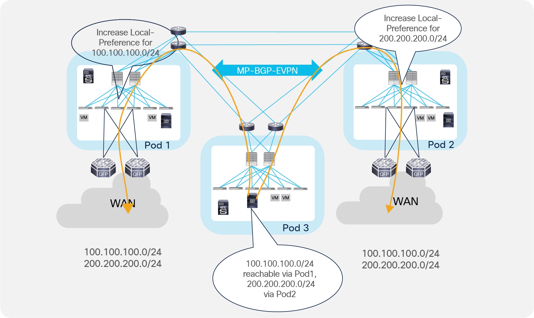
Influencing Outbound Traffic Flows by Tuning Local Preference
Notice that the behavior shown above for the endpoint in Pod 3 also applies to the endpoints deployed in Pod 1 and Pod 2. This means that all the outbound traffic destined to 100.100.100.0/24 that originated from endpoints connected to the ACI Multi-Pod fabric will always prefer the L3Out connection in Pod 1 independently from the specific Pod where those endpoints are connected (the same applies for traffic destined to 200.200.200.0/24 that will always prefer the L3Out connection in Pod 2).
Note: The statement above is always valid under the basic assumption that there are no endpoints directly connected to the Border Leaf nodes. This is because endpoints connected to the BL nodes will always prefer the local L3Out connection to communicate to all the IP prefixes received from the external routers when using OSPF or EIGRP as the routing protocol with the external routers. When using BGP, instead, the tuning of local-preference mentioned previously would also allow locally connected endpoints to prefer an L3Out located in a different Pod for all outbound communications.
If endpoints belonging to the same BD are connected across all the Pods of the Multi-Pod fabric, inbound traffic may be received via any of the deployed L3Out connections. This is the case assuming that the BD IP subnet is announced via all the L3Outs deployed across Pods (which is normally a best practice to provide resilient inbound paths) and may lead to the creation of the asymmetric communication behavior shown in Figure 44.
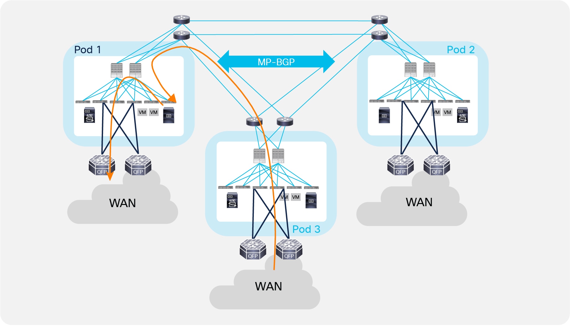
Asymmetric Inbound and Outbound Traffic Flows
The traffic pattern shown above causes problems when deploying stateful perimeter services (like firewalls) between the fabric and the WAN, so it is important in those case to maintain symmetry between inbound and outbound flows. This can be achieved in different ways, depending on the type of communication required with the external routed domain:
● For communication with the Internet, it is very common that the perimeter firewall perform NAT/PAT. This ensures that inbound and outbound flows always traverse the same FW device.
● For communication with private WAN networks, NAT/PAT is usually not used; in that case, the most common way of keeping inbound and outbound flows symmetric consists in advertising granular endpoint host route information into the WAN, as shown in Figure 45 below.
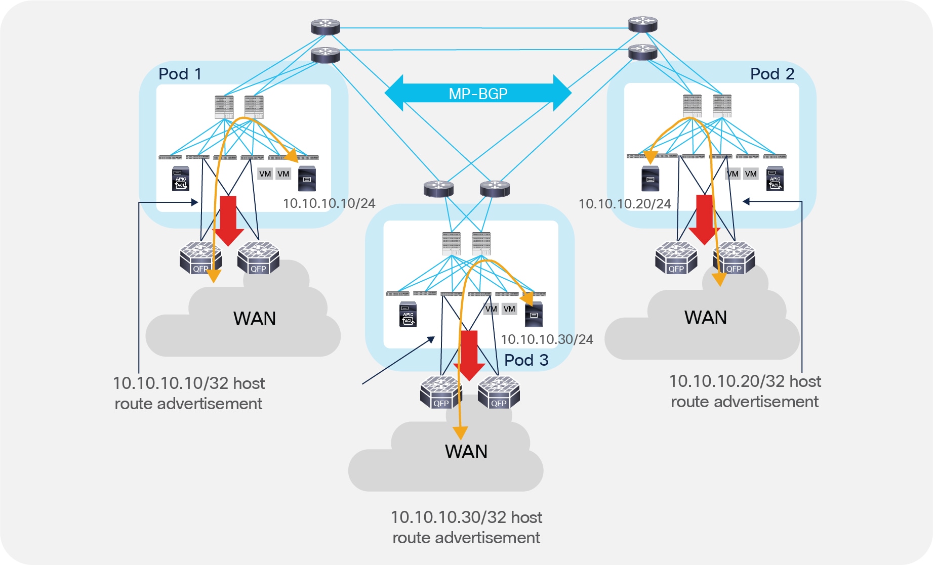
Making Inbound and Outbound Traffic Path Symmetric with Host Route Advertisement
The capability of advertising host routes via Border Leaf L3Out connections is available from ACI release 4.0. For earlier releases, the only option is deploying GOLF L3Outs, as discussed in the previously referenced Cisco Live presentation.
Alternatively, the recommendation is to cluster stateful network services deployed across Pods (either in an Active/Standby or Active/Active fashion), as discussed in more detail in the Network Services Integration section.
A specific use case is the one where different Pods are deployed inside the same DC location. In this case, it is typical to use a centralized connection toward the external network domain. As shown in Figure 46, the end result is that traffic from endpoints connected to all the Pods must be hair-pinned to the Pod externally connected (Pod 1 in the example below).
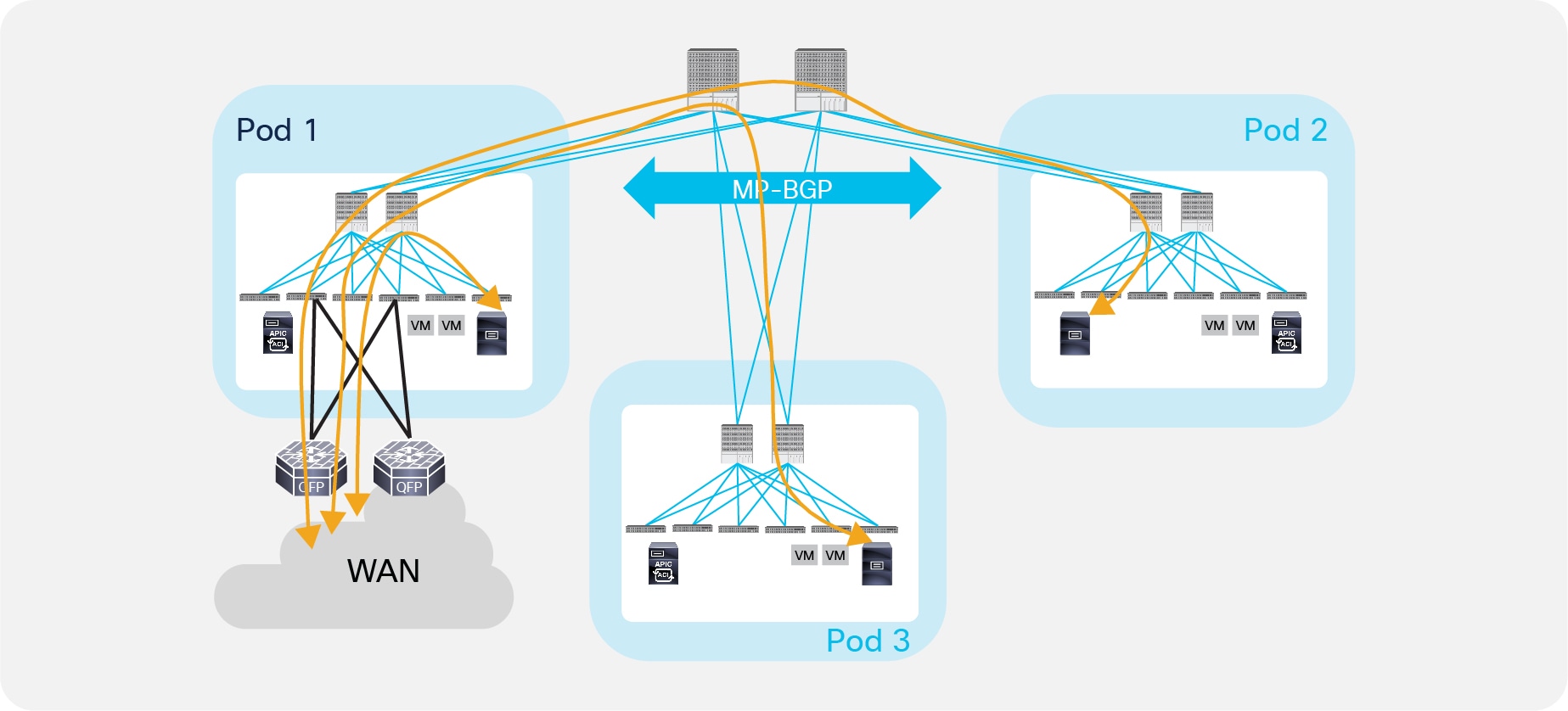
Centralized Access to the External Network Domain
This usually does not represent a concern, given the very low latency and available bandwidth between Pods deployed in the same physical DC location. At the same time, this model is not concerned by the creation of asymmetric traffic pattern, so integration of stateful services does not require any specific deployment or design considerations.
The integration of networks services with ACI can be done in different ways
● Using manual configuration of bridge domains and EPGs
● Using the service graph with the device package
● Using the service graph in unmanaged mode or network-only stitching mode
The decision on what approach to follow depends on several factors, including operational model choice, need for automation and availability of a device package for the device of choice. For more information and design guidance around the deployment of network services with ACI, please refer to the design guide below: https://www.cisco.com/c/en/us/solutions/collateral/data-center-virtualization/application-centric-infrastructure/white-paper-c11-734298.html.
As of Cisco ACI Release 3.2(2), the deployment options described here are available for integrating service nodes with Cisco ACI Multi-Pod fabrics (see Figure 47).
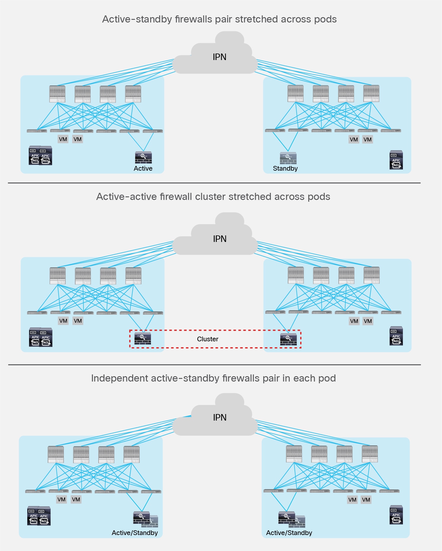
Network Services Deployment Options with ACI Multi-Pod Solution
● Active-standby firewalls pair-stretched across Pods: This model can be applied to both north-south and east-west traffic flows. This fail-safe model does not allow the creation of an asymmetric traffic path that could lead to communication drops. At the same time, because of the existence of a single active service node connected to the Multi-Pod fabric, this option has certain traffic-path inefficiencies, because by design some traffic flows will hair-pin across the Interpod Network (IPN). Therefore, you should be sure to properly dimension the bandwidth available across Pods and consider the possible latency impact on application components connected to separate Pods.
The active-standby model is supported with service nodes deployed in transparent or routed mode with independent L3Out connectivity of the external Layer 3 domain. Both the traditional Border Leaf nodes and the GOLF router options are supported for L3Out connectivity.
● Active-active firewall cluster stretched across Pods: beginning with ACI release 3.2(4d), an active/active FW cluster can be stretched across Pods. When deploying Cisco ASA or Firepower firewall appliances, this deployment model takes the name of “Split spanned Ether-channel” and ensures that all the nodes of the cluster “own” the same MAC/IP values so that the stretched firewall cluster appears as a single logical entity to the ACI Multi-Pod fabric. This deployment model removes any concern of creation of asymmetric traffic paths for both east-west and north-south traffic flows, as traffic will be dynamically redirected to the specific firewall node owning the connection state for that specific traffic flow. This option requires “anycast service” and PBR.
● Independent active-standby firewalls pair in each Pod: This model mandates that symmetric traffic flows through the service nodes be maintained because the connection state is not synchronized between independent nodes. This requirement can be achieved with the following approaches:
◦ You can deploy symmetric Policy-Based Redirection (PBR) for both north-south and east-west security policy enforcement. This approach is the recommended solution. It consists of defining a PBR policy that specifies multiple active service nodes. Cisco Nexus® 9000 Series Switches (EX platform or newer), used as leaf nodes, would then apply the symmetric PBR policy, selecting one of the available nodes for the two directions of each given traffic flow (based on hashing).
◦ The use of symmetric PBR mandates that the service nodes be deployed in routed mode only. This model can integrate with L3Out connectivity with traditional Border Leaf nodes or GOLF nodes for external Layer 3 connectivity.
◦ If deployment of symmetric PBR is not possible, in the specific case of perimeter firewall deployments (only for north-south traffic flows), it is necessary to keep ingress and egress traffic flows optimized and symmetric. This can be achieved by enabling granular host-route advertisement toward the external Layer 3 domain to ensure that ingress traffic paths are always delivered in the “right Pod” where the destination endpoint is connected. Prior to ACI software release 4.0, host-route advertisement is only supported on GOLF L3Out; firewall nodes can then be deployed in routed mode and physically connected north of the GOLF routers to apply policy on the traffic when it is not encapsulated by Virtual Extensible LAN (VXLAN).
◦ Support for host-route advertisement is extended to regular L3Outs deployed on Border Leaf nodes from release 4.0 onwards. This allows connecting firewall nodes deployed in routed mode between the Border Leaf nodes and the external WAN edge routers.
The options and considerations are summarized in Table 1.
Table 1. Service Node Integration Modes for Cisco ACI Multi-Pod Fabric
|
|
Active-standby firewall nodes stretched across pods (north-south) |
Active-standby firewall nodes stretched across pods (east-west) |
Active-active firewall cluster stretched across pods (north-south or east-west) |
Active-standby firewall nodes per pod (north-south) |
Active-standby firewall nodes per pod (east-west) |
| Transparent mode |
Yes |
Yes |
No |
No |
No |
| Routed mode |
Yes |
Yes |
Yes (from ACI 3.2(4d)) with anycast service and PBR |
Yes |
Yes |
For more information on how to integrate network services with an ACI Multi-Pod fabric please refer to the paper below: https://www.cisco.com/c/en/us/solutions/collateral/data-center-virtualization/application-centric-infrastructure/white-paper-c11-739571.html.
The introduction of a new solution like ACI Multi-Pod immediately triggers migration questions from an existing deployed infrastructure. The assumption in this section is that customers looking to deploy Multi-Pod are starting from an already deployed ACI fabric, so discussions on how to interconnect a legacy brownfield network to ACI is out of the scope for this paper.
Note: For more information on how to migrate existing networks to ACI please refer to the papers below:
https://www.cisco.com/c/en/us/td/docs/switches/datacenter/aci/apic/sw/migration_guides/migrating_existing_networks_to_aci.html.
Figure 48 shows the end goal of the procedure, which is migrating a single ACI fabric to Multi-Pod by adding an additional Pod to the fabric.
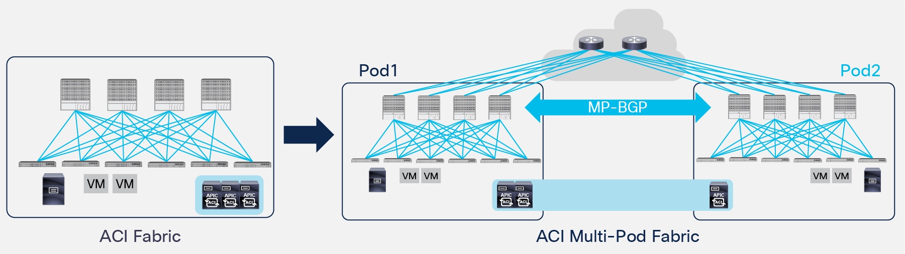
Migrating from ACI Fabric to ACI Multi-Pod Fabric
The following are the steps required to complete this migration process:
1. Preconfigure the IPN devices and their interfaces (IP addresses, MTU, DHCP-Relay, OSPF, PIM Bidir, etc.) to be able to connect to the spine nodes of the existing ACI Fabric and of all the additional Pods that need to be added to the Multi-Pod solution. As previously mentioned, this is a “Day 0” required configuration that is performed independently from ACI (the IPN devices are not managed by APIC) and that should not require any further change once it is put in place.
2. Upgrade the ACI fabric (leaf, spine and APIC nodes) to run the minimum ACI software release 2.0, which is a pre-requisite to support Multi-Pod.
Note: The recommendation is to run the same ACI software release across the Pods at steady state. It is, however, possible to run separate software versions during the initial addition of a remote Pod to the fabric or during the upgrade of a Multi-Pod fabric.
3. Connect the spines to the IPN devices, configure the IP addresses and enable OSPF for the spine interfaces (via APIC). At the end of this step, full IP reachability at the infrastructure level is obtained between the ACI fabric and the IPN devices.
4. Connect the spines in the new Pod to the IPN devices and similarly configure their interfaces via APIC. Powering up the spines in the new Pod would then allow this new Pod to ‘join’ the Multi-Pod fabric based on the procedure discussed in the “Pod Auto-Provisioning” section.
5. The final step is disconnecting one of the APIC nodes from Pod1 and connecting it to Pod2. The APIC node should be reset and the initial setup script should be run again to ensure it can get connected to the new Pod. It is worth noticing that an APIC node keeps the same IP address (assigned from the TEP Pool valid for the fabric it was initially connected).
The exact same procedure can be followed to migrate from an initial ACI Stretched Fabric to a Multi-Pod configuration, as shown in Figure 49.
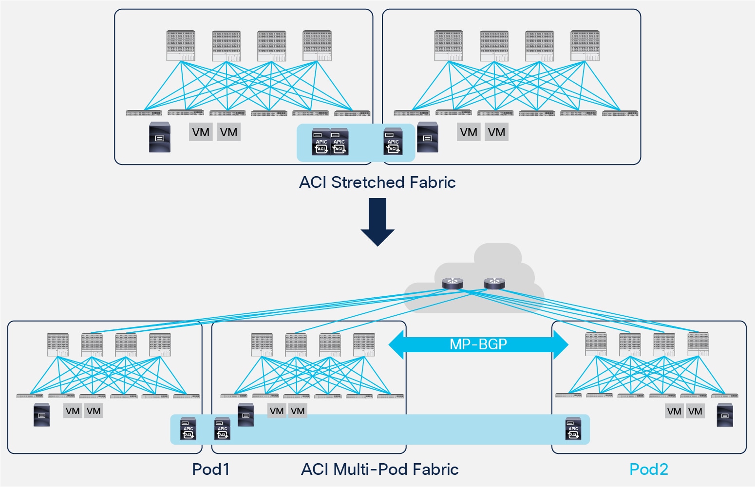
Migrating from ACI Stretched Fabric to ACI Multi-Pod
In the scenario above, the whole stretched fabric initially deployed is considered as a single Pod to which an additional Pod2 can be added to create a Multi-Pod fabric.
Specific considerations are instead required to migrate from ACI stretched fabric to ACI Multi-Pod by separating the original sites, as shown in Figure 50.
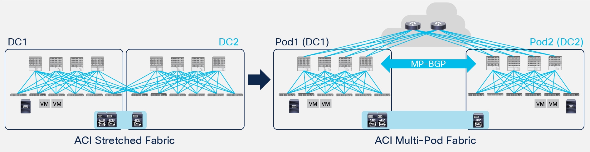
Migrating from Stretched Fabric to Multi-Pod by Separating the Original DCs
The fundamental issue with this migration approach is the fact that, as discussed in the “IPN Control Plane” section, the infrastructure IP addresses assigned to the leaf and spine nodes are carved from a unique TEP Pool assigned to the Pods they belong. Separate Pods use separate TEP Pools, as previously shown in Figure 8. This clearly is not the case with the ACI stretched fabric, since all the leaf and nodes are addressed from the same TEP Pool. As a consequence, separating the two sites initially connected in a stretched fabric design would require a complete reconfiguration for one of the two sites.
While this is doable by first moving all the active workloads to the first site, this procedure is considered very invasive and as a consequence it is not recommended nor supported by Cisco.
Cisco ACI Multi-Pod fabric represents the newest deployment option to interconnect ACI fabrics. The different Pods may represent different islands (rooms, halls) deployed in the same physical data center location, or could map to geographically dispersed data centers (up to 50 msec RTT latency).
In both use cases, Multi-Pod provides operational simplification by allowing a single APIC cluster to manage all the interconnected Pods. This characteristic also allows for the creation of a single policy domain across all the Pods, ensuring consistent end-to-end security policies.
ACI Multi-Pod represents the natural evolution of the original Stretched Fabric design, providing a more resilient deployment option through the isolation of fabric control protocol across different Pods (failure domain isolation across Pods). Various migration options have been internally validated and are available to drive the adoption of this new solution.