- Overview
- User Interface
- Plan Objects
- Traffic Demand Modeling
- Simulation
- Simulation Analysis
- Forecasting Traffic
- IGP Simulation
- MPLS Simulation
- Quality of Service Simulation
- BGP Simulation
- Advanced Routing with External Endpoints
- VPN Simulation
- Multicast Simulation
- Layer 1 Simulation
- Metric Optimization
- LSP Optimization
- SR-TE Optimization
- Changeover
- Reports
- Cost Modeling
- Plot Legend for Design Layouts
Cisco WAE Design 6.2 User Guide
Bias-Free Language
The documentation set for this product strives to use bias-free language. For the purposes of this documentation set, bias-free is defined as language that does not imply discrimination based on age, disability, gender, racial identity, ethnic identity, sexual orientation, socioeconomic status, and intersectionality. Exceptions may be present in the documentation due to language that is hardcoded in the user interfaces of the product software, language used based on RFP documentation, or language that is used by a referenced third-party product. Learn more about how Cisco is using Inclusive Language.
- Updated:
- July 31, 2015
Chapter: Simulation
Simulation
WAE Design network simulations calculate demand routings and traffic distributions through the network based on the given traffic demand, network topology, configuration, and state. Simulation is the fundamental capability of WAE Design on which most of the other tools are built, including those for planning, traffic engineering, and worst-case failure analysis. A number of protocols and models are supported, including IGP, MPLS RSVP-TE, BGP, QoS, VPNs, Multicast, and Layer 1 (L1).
This chapter focuses on the general features of WAE Design simulations. The individual protocols and models are described in their respective chapters.
Simulations can be performed under different simulation convergence modes (Fast Reroute, IGP and LSP Reconvergence, and Autobandwidth Convergence), depending on which stage of the network recovery after failure is being investigated. If in Autobandwidth simulation mode, the results for simulations with failures are identical to those in the IGP and LSP Reconvergence simulation mode. The default simulation mode is IGP and LSP Reconvergence, and except where identified, the documentation describes this simulation mode. For more information, see the MPLS Simulation chapter.
|
|
|
|---|---|
Traffic Demand Modeling chapter |
|
Fast Reroute, Autobandwidth Convergence, and Autobandwidth Convergence (Including Failures) simulation modes |
MPLS Simulation chapter |
IGP Simulation chapter |
|
MPLS Simulation chapter |
|
Quality of Service Simulation chapter |
|
BGP Simulation chapter |
|
VPN Simulation chapter |
|
Multicast Simulation chapter |
|
Layer 1 Simulation chapter |
|
Simulation Analysis chapter |
|
Forecasting Traffic chapter |
|
Metric Optimization chapter |
|
LSP Optimization chapter |
Simulation
WAE Design uses demands to simulate traffic between source and destination endpoints within a network. Each demand has a specified amount of traffic.
By default, an up-to-date simulation of an open plan is always available. Any change in the plan that affects or invalidates the current simulation automatically triggers a resimulation. Types of changes that result in re-simulations are those that would typically affect routing in a network.
- Changes in topology, such as adding and deleting objects or changing explicit paths.
- Changes to an object’s state, such as failing an object or making it inactive.
- Changes in numerous properties, such as metrics, capacities, and delay.
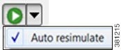
To toggle automatic resimulation on and off, follow one of these two steps.
- Select the drop-down arrow next to the Simulation On/Off icon (white arrow in green circle) in the Visualization toolbar. Click the “Auto resimulate” option to toggle it on and off.
State
The state of an object affects simulation and determines whether an object is operational.
- Failed State —Identifies whether the object is failed. See the Failed State section.
- Active State —Identifies whether the object is available for use in the simulated network. For example, an object might be unavailable because it has been set administratively down. See the Active State section.
- Operational State —Identifies whether an object is operational. For instance, an object might be non-operational because it is failed, is inactive, or because other objects on which it depends are not operational. See the Operational State section.
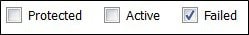
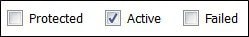
The Failed and Active columns in the tables show a visual representation of their status. Likewise, you can show the Operational column to show the calculated operational state. In each column, T means the object is in that state and F means it is not. Note that the T or F for Active state in the Interfaces table is reflective of the associated circuit. The plot shows graphical representations of these states with crosses of various colors and fills.

Note![]() For detailed information about visual representations of failed and inactive states in the L1 view, see the Layer 1 Simulation chapter.
For detailed information about visual representations of failed and inactive states in the L1 view, see the Layer 1 Simulation chapter.
Failed State
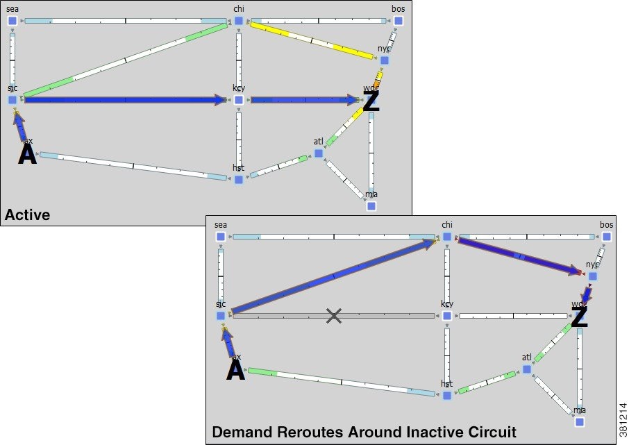
The quickest way to see the effects of failures in a Simulated Traffic view is to have demands in place and then fail an object. The plot immediately displays where the traffic increases as a result (Figure 5-1), and the Util Sim column in the Interfaces table reflects the traffic changes. Demands are then rerouted around the failure (Figure 5-2).
To specify that a demand should not reroute around failures, deselect the Reroutable option in the demand’s Properties dialog box. This can be used as a way of including L2 traffic on an interface. For example, a one-hop, non-reroutable demand can be constructed over the interface to represent the L2 traffic. Other, reroutable, demands, can be constructed through the interface as usual. If the interface fails, the L2 traffic is removed and the L3 traffic reroutes.
You can simultaneously fail one or more objects of the same type. If you select an interface to fail, you are actually failing its associated circuit.
|
|
|
|---|---|
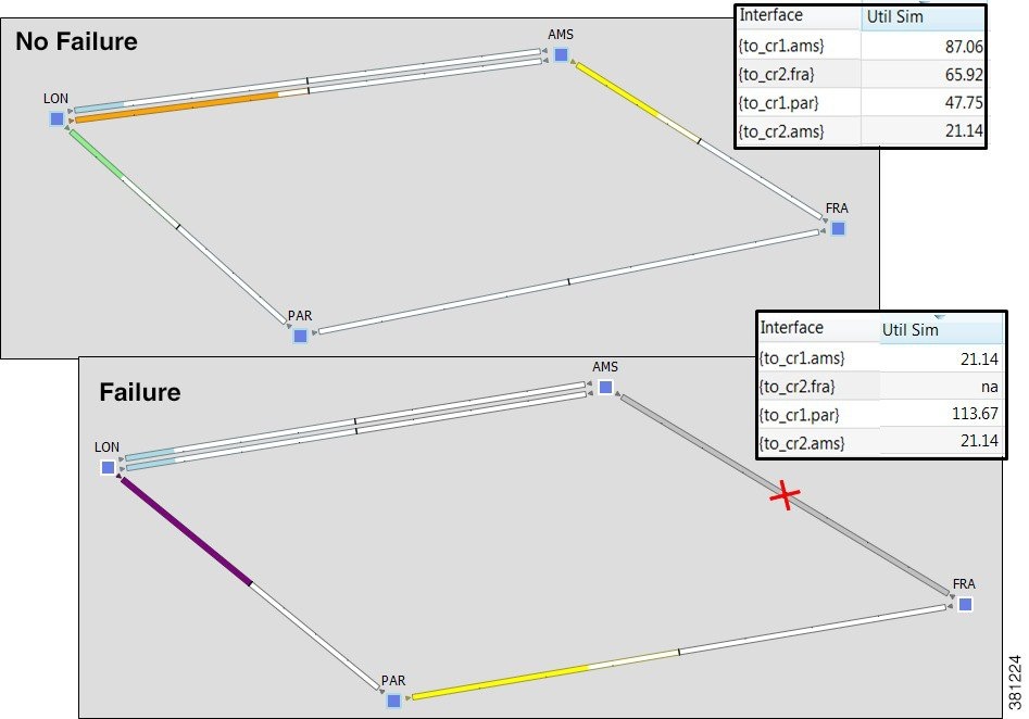
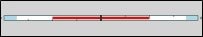
Figure 5-2 Reroute of Demand Around Failed Circuit
Failures in the Network Plot
In the network plot, a solid red X appears to show failure.
|
|
|
|---|---|
|
|

|
|

|
|

|
One or more sites, nodes, or circuits within the site failed. |
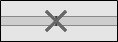
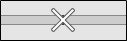
For failed ports or port circuits that do not take down the entire circuit, a circuit with a red strikethrough line in the middle shows the reduced capacity.
|
|
|
|---|---|
|
The circuit is a LAG, and one or more ports or port circuits in the LAG failed.The red strikeout line is the percent of unavailable capacity due to the failure. |
Fail and Recover Objects
Protect Circuits within SRLGs
You can protect circuits from being included in SRLG failures and SRLG worst-case analysis, though there are differences in behavior, as follows.
- These circuits do not fail if you individually fail an SRLG as described in the above steps. However, if you fail the circuit itself, it will fail.
- These circuits are protected from being included in Simulation Analysis regardless of whether they are in an SRLG or not. For more information, see the Simulation Analysis chapter.
Note that this setting has no effect on how FRR SRLGs are routed. For information on FRR SRLGs, see the MPLS Simulation chapter.
Step 1![]() Set the Protected property for circuits.
Set the Protected property for circuits.
a.![]() Select one or more circuits.
Select one or more circuits.
b.![]() Right-click a selected circuit, and select Properties from the context menu.
Right-click a selected circuit, and select Properties from the context menu.
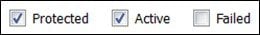
c.![]() Select the Protected option, and click OK.
Select the Protected option, and click OK.
Step 2![]() Set the Network Option property for protecting circuits included in SRLGs.
Set the Network Option property for protecting circuits included in SRLGs.
a.![]() Select the Edit->Network Options menu or the Network Options icon from the Visualization toolbar.
Select the Edit->Network Options menu or the Network Options icon from the Visualization toolbar.
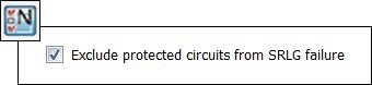
c.![]() Select the option to exclude protected circuits from SRLG failures, and click OK.
Select the option to exclude protected circuits from SRLG failures, and click OK.
Active State
An active/inactive state identifies whether an object is available for measured or simulated traffic calculations. An object can be inactive for one of three reasons.
- It is administratively down.
- It is a placeholder. For instance, you might be planning to install an object and want its representation in the network plot.
- It exists in a copied template plan, but was not in the original plan that was discovered.
You can simultaneously change the active state of one or more objects. If you change the active state of an interface, you are actually changing its associated circuit.
|
|
|
|---|---|
Like failures, changing an object from active to inactive immediately affects how demands are routed, and affects the Util Sim column in the Interfaces tables (Figure 5-3).
Inactive States in the Network Plot
In the network plot, a solid black X appears to show an inactive state.
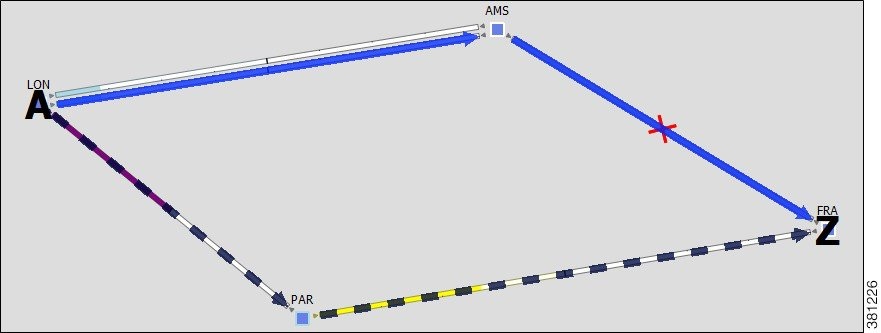
If a demand is inactive, the plot shows the ingress and egress sites marked with A and Z, respectively, but the demand (blue) path between them does not appear.
The inactive state takes precedence over a failure. For example, if a circuit is not active and then you fail it, the circuit continues to show a black X on it.
|
|
|
|---|---|
|
|

|
|

|
|

|
One or more sites, nodes, or circuits within the site are inactive. |
If a port or port circuit is inactive, a circuit with a black strikethrough line in the middle shows the reduced capacity.
Set Active or Inactive States
Step 1![]() Right-click one or more like objects from their respective tables. The Properties dialog box appears.
Right-click one or more like objects from their respective tables. The Properties dialog box appears.
Step 2![]() Click the Active check box to toggle it on or off. A check mark means the object is active.
Click the Active check box to toggle it on or off. A check mark means the object is active.
Operational State
The operational state identifies whether the object is functioning. You cannot set an operational state; rather, it is automatically calculated based on the failed and active states.
- Any object that is failed or inactive is operationally down.
- If the object relies on other objects that comprise it to be functioning, then its operational state mirrors the state of those objects.
|
|
|
|---|---|
Non-Operational Due to Failures
A red X with a white interior shows that an object is operationally down because of a failure of other objects. For example, if a node fails, a red X appears on the node itself and a red X with a white interior appears on all circuits to which it is attached.


Non-Operational Due to Inactive States
A black X with a white interior shows that an object is operationally down because of an inactive state of other objects. For example, if a node is inactive, a black X appears on the node itself and a black X with a white interior appears on both circuits to which it is attached.


Simulated Capacity
The Capacity column displays the configured physical capacity of interfaces, circuits, ports, and port circuits. Each circuit, port, and port circuit has a physical capacity that you can set in the Capacity field of the Properties dialog box. The interfaces have a configurable capacity that you can set in the Configured Capacity field. From these properties, a simulated capacity is derived for each object.
The Capacity Sim column is the calculated capacity of the object given the state of the network, which could include failures that reduce capacity. All utilization figures in the Interfaces, Circuits, and Interface Queues tables are calculated based on this Capacity Sim value. When referencing the Capacity Sim value, there are a few rules to note regarding its calculation.
- If a circuit’s capacity is specified, this becomes the simulated capacity of the circuit, and all other capacities (interface and constituent port capacities) are ignored. Specifying circuit capacities (rather than interface capacities) is the simplest way to modify existing capacities, which is useful, for example, for build-out planning.
- A circuit Capacity Sim is the same as the Capacity Sim for each of its constituent interfaces.
- If the circuit capacity is not specified, then the associated interface Capacity Sim values are the minimum of the configured interface capacity and that of its connected remote interface. Thus, the circuit capacity is effectively negotiated down to the minimum of the two interface capacities.
- If two ports are connected by a port circuit, then the Capacity Sim of the two ports and of the port circuit is set to the minimum capacity of the three, which again, effectively negotiates down the capacity of each side of the connection.
- In a LAG interface, if any of the constituent ports are operationally down, then the interface Capacity Sim column displays a value that is reduced by the aggregate capacity of all the ports that are down. For example, if a 1,000 Mbps port of a four-port 4,000-Mbps LAG is operationally down, the simulated capacity for that LAG interface becomes 3,000 Mbps.
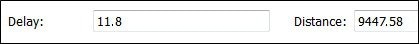
Simulated Delay and Distance
Both Delay and Distance are properties that can be set in the circuit Properties dialog box. To automate the process of setting these, use the Latency and Distance Initializer. For information, see the Latency and Distance Initializer section.
All WAE Design delay calculations that use the L3 circuit delay, such as Metric Optimization, use the Delay Sim value.
For more information on the delay and distance of L1 objects, see the Layer 1 Simulation chapter.
Latency and Distance Initializer
Following is the default behavior for the Latency and Distance Initializer. Note that if there are no Longitude and Latitude available for use by the initializer, The Distance and Delay properties are set to zero.
–![]() The current L1 circuits Delay and Distance properties are removed unless the “Keep existing distances if available” option is selected.
The current L1 circuits Delay and Distance properties are removed unless the “Keep existing distances if available” option is selected.
–![]() The L1 node and L1 waypoint Longitude and Latitude properties are used to estimate the L1 distances. If an L1 node does not have these properties set, the shortest distance calculation is based these same properties of its immediate parent site, if applicable. (L1 nodes are not required to have parent sites.) The L1 link delays are calculated from these distances.
The L1 node and L1 waypoint Longitude and Latitude properties are used to estimate the L1 distances. If an L1 node does not have these properties set, the shortest distance calculation is based these same properties of its immediate parent site, if applicable. (L1 nodes are not required to have parent sites.) The L1 link delays are calculated from these distances.
–![]() Each L1 circuit path’s Distance Sim and Delay Sim columns are calculated as the sum of the distances and delays of L1 links over which the L1 circuit path is routed.
Each L1 circuit path’s Distance Sim and Delay Sim columns are calculated as the sum of the distances and delays of L1 links over which the L1 circuit path is routed.
–![]() L3 circuit delays and distances are inherited from L1 circuits if there are L1 circuits mapped to the L3 circuits. Otherwise, the L3 delay and distance are estimated using the shortest distance between nodes at the endpoints of the circuits. If a node does not have Longitude and Latitude properties, the calculation is based on these same properties of its immediate parent site, if applicable. (Nodes are not required to have parent sites.) Thus, if you have an L1 model, the delays and distances are more precise because the physical paths that the L3 circuits take are known.
L3 circuit delays and distances are inherited from L1 circuits if there are L1 circuits mapped to the L3 circuits. Otherwise, the L3 delay and distance are estimated using the shortest distance between nodes at the endpoints of the circuits. If a node does not have Longitude and Latitude properties, the calculation is based on these same properties of its immediate parent site, if applicable. (Nodes are not required to have parent sites.) Thus, if you have an L1 model, the delays and distances are more precise because the physical paths that the L3 circuits take are known.
–![]() ITU G.826 adjustments are used to convert L3 circuit distance (d) to an adjusted circuit distance (r) as follows.
ITU G.826 adjustments are used to convert L3 circuit distance (d) to an adjusted circuit distance (r) as follows.
If this option is unchecked, set r equal to d.
- Both the L3 and L1 delays are calculated to be the speed of light along a distance r, multiplied by the speed of light in medium correction factor (between 0 and 1). The default for this correction factor is 0.67.
Step 1![]() This initializer can act on two different selected object types (L1 links and L3 circuits), so the defaults for the dialog box differ, depending both on selections and on how you access it. Regardless of the method, you can modify your selection options once the dialog box is opened. Following are guidelines for having the dialog box open with the most desirable defaults.
This initializer can act on two different selected object types (L1 links and L3 circuits), so the defaults for the dialog box differ, depending both on selections and on how you access it. Regardless of the method, you can modify your selection options once the dialog box is opened. Following are guidelines for having the dialog box open with the most desirable defaults.
|
|
|
|
|---|---|---|
Right-click an L1 link, and select Initialize Latency from the context menu. |
||
Step 2![]() In each section, Layer 1 and Layer 3, verify or change your selection to act on the desired objects.
In each section, Layer 1 and Layer 3, verify or change your selection to act on the desired objects.
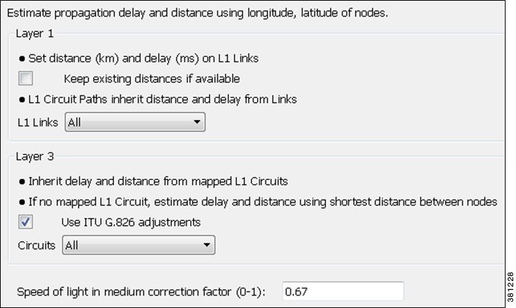
- For L1 links, the default is to delete distances. To keep them, select the option to keep existing distances.
- For L1 circuit paths, the default is to inherit distance and delay from L1 links. If desired, use the L1 Links drop-down list to base these calculations on all, selected, or tagged L1 links. If you do not want the distance and delay set on L1 circuit paths, select None.
- For L3 circuits, if desired, use the Circuits drop-down list to calculate L3 circuit delay and distance for all, selected, or tagged L3 circuits. If you do not want the delay or distance set on L3 circuits, select None.
Verify the inclusion ITU G.826 adjustments in the calculation, which is the default and which is usually left unchanged.
Step 3![]() For both L1 links and L3 circuits, verify or change default speed of light factor of 0.67. This is usually left unchanged.
For both L1 links and L3 circuits, verify or change default speed of light factor of 0.67. This is usually left unchanged.
 Feedback