Cisco Crosswork Hierarchical Controller 7.1 Network Visualization Guide
Available Languages
Bias-Free Language
The documentation set for this product strives to use bias-free language. For the purposes of this documentation set, bias-free is defined as language that does not imply discrimination based on age, disability, gender, racial identity, ethnic identity, sexual orientation, socioeconomic status, and intersectionality. Exceptions may be present in the documentation due to language that is hardcoded in the user interfaces of the product software, language used based on RFP documentation, or language that is used by a referenced third-party product. Learn more about how Cisco is using Inclusive Language.
- US/Canada 800-553-2447
- Worldwide Support Phone Numbers
- All Tools
 Feedback
 Feedback
Discovery and Visualization Applications and Feature Set
The following table lists the Crosswork Hierarchical Controller discovery and visualization applications. The Legend column indicates if the application/feature falls into one of the following categories:
● Common: Common to all layers and multi-layer
● IP: Relevant to IP links and services
● Optical: Relevant to fibers, optical links, OTN/ETH connections
Table 1. Applications and Feature Set
| Category |
Application name |
Legend |
Description |
| Discovery and Visualization |
Common |
Visualize IP and optical links/tunnels/services between geo sites on a satellite or schematic map, with correlation between layers. |
|
| Common |
Go back in time to a date in the past and analyze the network as it was at that point in time. |
||
| Common |
Show relationships between links in different layers (for example, show all SR policies over all or specific physical links). |
||
| Common |
Show full tabular view of devices, sites, links, connections, services, cards, ports, transceivers, power supplies, fans, and shelves |
||
| Common |
View visual widgets displaying inventory, topology, and services info. Define rule-based widgets with SHQL queries. |
||
| Common |
Analyze historical records of all inventory resources, topology, and service changes (add, modify, and delete). |
The following terms are used interchangeably throughout the guide.
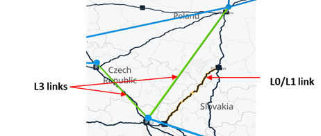
● Optical and L0/L1 (Layer 0/Layer 1)
● IP/MPLS and L3 (Layer 3)
| Acronym |
Definition |
| AGG |
Aggregation |
| ARP |
Address Resolution Protocol |
| CMD |
Command key on a Mac |
| CTRL |
Control key on Windows |
| EMS |
Element Management System |
| ETH |
Ethernet |
| Gbps |
Gigabits per second |
| IGP |
Interior Gateway Protocol |
| IP |
Internet Protocol |
| L0 |
Layer 0 |
| L1 |
Layer 1 |
| L3 |
Layer 3 |
| LAG |
Link Aggregation Group |
| LOG |
Logical |
| LSP |
Label-Switched Path |
| MPLS |
MultiProtocol Label Switching |
| NMS |
Network Management System |
| OCH |
Optical Channel |
| ODU |
Optimized Distribution Unit |
| OEO |
Optical-Electrical-Optical |
| OMS |
Optical Monitoring System |
| ONE |
Optical Network Element |
| OPS |
Optical Packet Switching |
| OTS |
Optical Transmission Section |
| OTU |
Optical Test Unit |
| PHY |
Physical |
| QoS |
Quality of Service |
| SDN |
Software-Defined Networking |
| TE |
Traffic Engineering |
| UI |
User Interface |
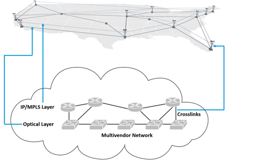
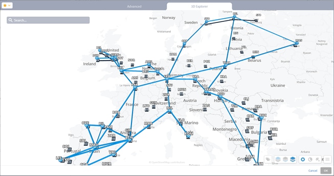
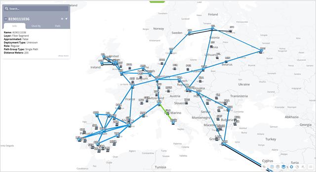
Cisco Crosswork Hierarchical Controller Explorer depicts a model of a multilayer, multi-vendor network that enables you to explore the relationship between the Optical layer and the IP/MPLS layer. The way this relationship is realized is through the discovery and visualization of the crosslinks that connect the layers.
The network map (model) displays L0-L3 topology and L0-L3 failures. To review this information and the multilayer relationships, you can show this network map as only the Optical layer, IP/MPLS layer, or both layers. Further exploration includes the ability to view intra-site connectivity and to drill down to specific object information, including crosslink port connectivity and multilayer paths.
This multilayer perspective enables you to better communicate with other network planners, operators, and architects within the company, as well as to answer critical questions about the network.
● What are the LSP (MPLS tunnel) paths?
● How many router hops are the LSPs taking and are they using optical resources efficiently?
● How are the L3 interfaces connected to the L0/L1 ports?
● How will a failure or temporary maintenance activity at the Optical layer impact service delivery at the IP/MPLS layer?
● How do I make sure that diversity is enforced for specific links or services?
● How do I detect proximity violations between fibers
● How do I check that planned path for new OMS is diverse from other OMSs
● Where are the optical vendors connected in the network?
● What is the intra-site connectivity within a site, such as within a metro area?
● What is the per-port connectivity in L3 link bundles?
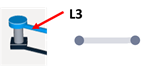
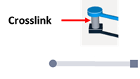
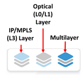
Figure 1 shows a representation of how the multiple layers and the crosslink appear in the three-dimensional network map. The IP/MPLS layer is on top, the Optical layer is on bottom, and the crosslink connects the two.
Note: The frequency of the network model updates is dependent on your configuration. For information on how often your model is updated, contact your system administrator or Cisco support representative.
Network Model Shown in Crosswork Hierarchical Controller Explorer UI
Note: While this guide describes full functionality, feature availability depends on your configuration.
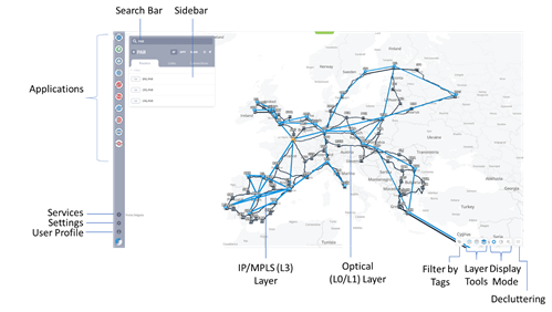
This section describes the basic tools for using and understanding the 3D Explorer UI. These tools are pervasive throughout the UI. Detailed descriptions of features, such as objects and in-depth exploration, are described throughout the remainder of the guide. There are two ways of exploring networks in 3D Explorer: the network map and the sidebar.
● Network Map — Shows one or more layers of the network with a geographic outline as a background. Each site is placed according to the longitude and latitude of the ONEs (optical network elements) and IP/MPLS routers within it. All objects (sites, routers, ONEs, links, and crosslinks) are visualized as an aggregate view. For detailed information, see Network Map.
● Live — Enables you to view the network on a specified date.
● Filter by Tags — Enables you to filter by tags such as vendor and region. For more information, see Network Map.
● View Layers — Enables you to view the Optical layer, IP/MPLS layer, or both. For more information, see see Network Map.
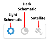
● Display Mode — Enables you to toggle the display between dark and light schematic modes or the satellite map. For more information, see Network Map.
● Search Bar — Located at the top left of the network map, the Search bar enables you to search the network for links, sites, network elements, etc.
● Sidebar — Enables you to drill down to more detailed information than what is available in the network map. For basic use, see Sidebar. More detailed use is described throughout the guide.
● Application Icons — Located on the left of the screen, these icons enable you to access the applications installed in your system. The following applications are available but if an application is not installed in your system, the icon does not appear.
◦ Explorer — Visualize IP and optical links/tunnels/services between geo sites on a satellite or schematic map, with correlation between layers. Using the time machine, go back in time to a date in the past and analyze the network as it was at that point in time.
◦ SHQL Dashboard — View visual widgets displaying inventory, topology, and services info. Define rule-based widgets with SHQL queries. See SHQL Dashboard.
◦ SHQL Query — Simple, yet sophisticated multi-layer query language to get inventory, topology, tunnels, and services. All based on multi-layer correlation.
◦ Network Inventory — Show full tabular view devices, sites, links, connections, services, cards, ports, transceivers, power supplies, fans, and shelves. See Network Inventory.
◦ Performance — For IP, view traffic utilization and OAM PM of port, links, tunnels and VPNs. Group links by topology context (all LAG members, between router A to B). Predict packet traffic utilization. For optical, show L0-L1 performance, including the correlation between photonic and L1 layer. View power level across a span of ROADMs and Amplifiers.
◦ Service Assurance — Visualize L1-L2-L3 service configuration and underlay path, with UNIs performance and events history.
◦ RCA (Root Cause Analysis) — Show which services and links in the upper layers were impacted by a lower layer link failure, especially in the case of a multi-layer where an optical link failure impacted IP links and services.
◦ Layer Relations — Show relationships between links in different layers (for example, show all SR policies over all or specific physical links). See Layer Relations.
◦ Network History — Analyze historical records of all inventory resources, topology, and service changes (add, modify, and delete).
◦ SHQL Widgets — Create SHQL widgets for the SHQL Dashboard.
◦ Shared Risk Analysis — Find if there are commonly shared resources (node, site, link, and card) between selected group of links in any layer. Group can be selected explicitly or as an SHQL rule.
◦ Network Vulnerability — Find if there will be network routing parts that will be isolated from the rest of the network given current failures and simulated failures.
◦ Failure Impact — Plan a maintenance event, finding which connections will be impacted by taking resources down and if there is an alternative path. When found, comparing existing and alternative path latency, cost, and hops. Supported for OTN, ETH, RSVP-TE tunnels.
◦ Path Analysis — Calculate, on demand, an IGP path between two routers, visualize the path, and show performance of IP links across the path.
◦ Path Optimization — Select a group or specific tunnels or connections and run a path calculation to optimize their path. Show results by comparing existing to optimized path based on latency, hops, and cost. X xApplies to OTN/ETH connection, RSVP-TE and SR policies, and VPNs.
◦ Services Manager — Service CRUD, show and provision all service types as listed above. For IP , L2-L3-VPNs, RSVP-TE, and SR policies. For optical, ETH/OTN connections, OCH, and ZR links.
◦ Link Assurance — Visualize RON link across ZR and OLS with performance in all layers.
● Services — Enables you to view system info, manage security settings and import or export Crosswork Hierarchical Controller settings.
◦ Model Settings — Add external data and tag resources based on rules.
◦ Device Manager — Manages Crosswork Hierarchical Controller southbound adapters, enabling you to add and manage devices, manage the assignment of devices to an adapter and monitor the adapter’s health as well as the devices topology and discovery states.
● Settings — Enables you to view system info, manage security settings and import or export Crosswork Hierarchical Controller settings.
● User Profile — Displays the name of the person logged in to the local Crosswork Hierarchical Controller Explorer. You can also change your password and logout of the Crosswork Hierarchical Controller Explorer UI in this area.
Crosswork Hierarchical Controller Explorer UI
By default, the map is configured for two layers. The number of layers can be customized, up to four layers by Cisco. for example, the OMS layer and the OTN layer may be displayed for the optical network.
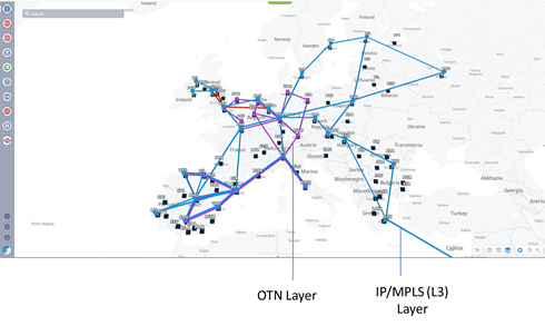
3D Explorer UI – 3 Layers
An object is any logical or physical network component that is available for exploration or visualization in the Explorer UI. These include the following, and each is defined throughout the guide.
● IP/MPLS—Routers, L3 links, logical and physical interfaces, and LSPs
● Optical—ONEs, L0/L1 links, ports, and connections
● Multilayer—Crosslink, sites
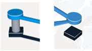
While there are many object icons, the basic premise is that routers appear as circle icons and ONEs appear as square icons. With this knowledge, you can interpret most icons in the UI. For a complete list of icons, see Legend.
Example: You immediately know that all icons in Figure 4 represent crosslinks because they each contain a router (circle) and a ONE (square). When you select the crosslink, it appears in orange.

Crosslink Icons
This legend helps you quickly identify icons. Detailed descriptions of them are throughout the guide.
● Layer 3
Tip: Remembering that a circle is always an L3 router and that a square is always an L0/L1 network element enables you to easily identify most other icons.
| Icon |
Description |
|
|
L3 router |
|
|
Network map showing a site containing at least one router in the IP/MPLS layer view. If all layers are visible, site in network map that contains only routers whether directly or indirectly with nested sites containing only routers. |
|
|
L3 link |
|
|
L3 link bundle |
| Icon |
Description |
|
|
ONE |
|
|
Network map showing a site containing at least one ONE in the Optical layer view. If all layers are visible, site in network map that contains only ONEs whether directly or indirectly with nested sites containing only ONEs. |
|
|
L0/L1 link |


| Icon |
Description |
|
|
Crosslink (link between a router and a ONE) |
|
|
Site in network map that contains at least one router, at least one ONE, and at least one crosslink connecting a router and ONE, whether directly or due to nested sites within it. If a crosslink has not been discovered yet, the site temporarily appears without it. |
The sidebar enables you to view details of the network map. The information is organized in a hierarchical format, enabling you to drill down to more details for each object.
To open the sidebar, select an object from the network map.
● If you select a site, the sidebar opens to show all objects within the site and all multilayer options. If you select a grouped site, the sidebar lists all objects of all sites contained within the grouped site.
● To see details about any given object, select the applicable tab and then select the object.
● For more information on grouped sites, see Network Map. For more information on exploring data in the sidebar, see Multilayer Crosslinks, IP/MPLS Layer and Multilayer Paths, and Optical Layer and Multilayer Paths.
● If you select an L3 link or L0/L1 link, the sidebar opens to show all L3 links or all L0/L1 links going between the two sites on each end of the link.
If you select the icon to the left of the object name in the sidebar, you can show the type of inventory item you are currently viewing.
Show Inventory Item
Select the object for which you need information. Each time you select a different object, all content in the sidebar updates to apply only to that object.
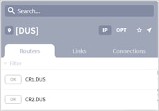
● If you select a site object, the Sidebar includes tabs for IP and Optical devices and cross links on that site. Click the IP tab to get more details of the routers at the site together with their links and connections. Click the OPT tab to get more details of the nodes at the site together with their links and connections. Click the XLNK tab to get more details on the cross links.
● If you select a crosslink, the Sidebar displays details of the crosslink, its connections and path.
● If you select an optical node, the Sidebar displays details of the node together with its links and connections. If viewing a path, such as an LSP path or the optical path that an L3 link or LSP path takes, moving the cursor between the routers or between the ONEs shows the link names.
Example: Figure 6 and Figure 7 show the MIL site information on the left. All links and LSPs accessed from here are applicable to any given router within the MIL site. Figure 8 shows selecting the CR1.MIL router to open information specific to that router. Then selecting the Links tile shows all links connected to the CR1.MIL router. Figure 9 shows a continuation of drilling down for more information by selecting an L3 link and then selecting the Paths tile to view the associated multilayer path.
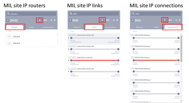
Example of Site IP Links and Connections
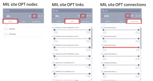
Example of Site OPT Links and Connections

Example of Drilling Down to a Router
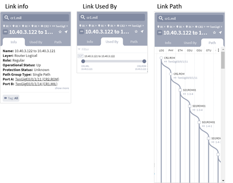
Example of Drilling Down in a Link
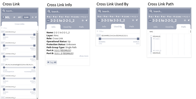
Example of Drilling Down in a Cross Link
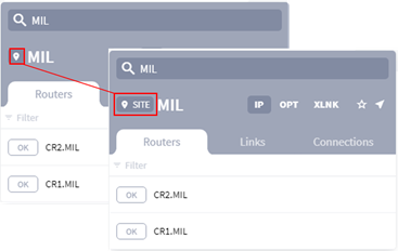
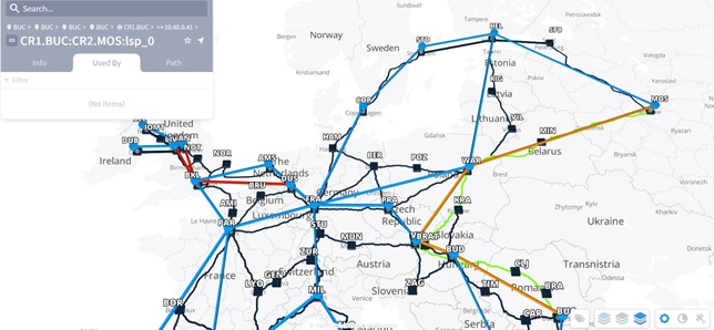
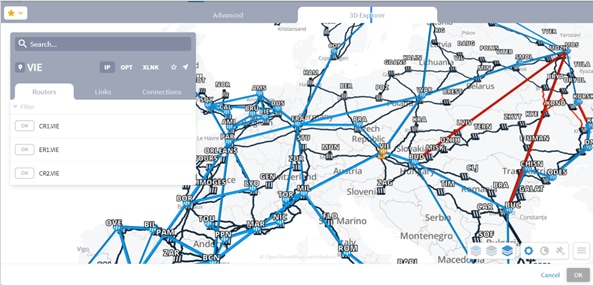
The Search feature finds all objects whose name includes the search string, including crosslinks and both layers. Once the results are displayed, select the object for which are you looking, and it will then appear in the sidebar.
Start typing and as you type, the results narrow to fit the string. The input is not case-sensitive. You can use an asterisk (*) or a question mark (?) as a wildcard between two strings. An * may be used to represent any number of characters, whereas a ? represents one character.
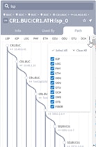
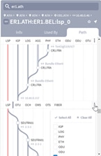
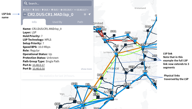
The left side of Figure 11 shows a search for all instances of the string MIL, which locates multiple objects using this search criteria. The right side shows a search for all strings containing CR1 + <all strings> + MIL (in that order), which locates the relevant LSPs.
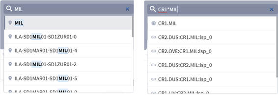
Example Searches
Filtering finds all instances of a name within the content that is displayed in the sidebar. For instance, if you are in the Routers tab, the filter only finds router names.
In the Filter text box, start typing and as you type, the results narrow to fit the string. The input is not case-sensitive. You can use an asterisk (*) as a wildcard between two strings.
Example: Figure 12 shows an unfiltered list of LSPs in a site (left) and a filter of an LSP on the site that has the number 142 as part of its name.
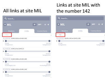
Example Filters
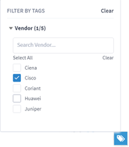
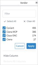
You can also filter by tags such as vendor/provider or region. Tags appear as filters and as attributes in the sidebar.
These tags are added using the REST API or the Model Settings application. For more information, see the Cisco Crosswork Hierarchical Controller Administration Guide. From version 5, tags can be attached to all types of resources.
The filtering system applies an OR to all selected values of a tag and an AND between tags.
For example, assuming these tags have been defined and assigned to routers:
● [x] Cisco
● [ ] Juniper
● [x] Huawei
Function
● [ ] Core
● [x] Edge
This filter matches (Vendor = (Cisco OR Huawei)) AND (Function = Edge).
That is, for a list of routers, the filter only shows Cisco Edge routers and Huawei Edge routers.
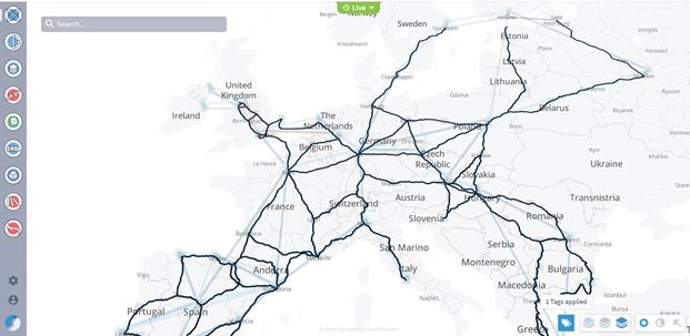
Example: Figure 13 and Figure 14 shows the filtered map with Cisco components.
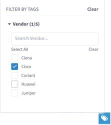
Filter by Tags
Viewing the Network Map
| To |
Do This |
| Expand grouped sites (sites containing other sites) to view their contents or to collapse these grouped sites into one. Parent sites are indicated with stripes.
|
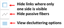
Use the mouse scroll wheel to zoom in or out. Zooming in expands the grouped sites. Zooming out collapses them. Note that zooming in also enlarges the map. To declutter the map, when zooming in to a target area, if both ends of the link appear in the target area, the link remains visible. If only one end of a link is in the target area, the link may be hidden (if the decluttering option is selected). However, if a link is currently selected, it will always appear even if only one end is in the target area. To find a specific site, click and hold the map while dragging it to the location of that site. |
| View a flat network map as if looking down on it from above, and to move the network map horizontally or vertically. This is useful for when zooming in to see details of grouped sites |
To move the network map, left-click and hold the cursor while dragging the network map horizontally or vertically. To zoom in or out, use the mouse scroll wheel. |
| Rotate the network map in a circular manner. For example, you could rotate the network map view so that the western view is at the forefront. This could be useful when exploring a specific region of the network map. |
Right-click and hold the network map while dragging it left or right to rotate it in that direction. Move the cursor vertically to view the network map in 3D. |
| Rotate the network map horizontally or vertically to see it in 3D, as a flat view (looking from the side or top), or as perspectives anywhere between the two. |
Right-click and hold the cursor while dragging the network map horizontally or vertically. |
| Filter by tags such as vendor/provider or region. Tags can be attached to any type of resource. |
Select the filter by tag icon.
|
| Show one or more network layers. |
Select the applicable network layer icon.
|
| Show dark and light schematic modes or the satellite map. |
Select the required icon.
|
| Reset the network map to the center of the page and show an aerial view of it |
Double-press the space bar. |
| Decluttering options: Hide links where only one side is visible. Hide passive fibers (with no OMS links above it).
|
|
Working with Objects and Views
| To |
Do This |
| Select an object. For information on objects, see Network Map. |
Click on the object. Selected objects are highlighted in orange. If applicable, associated links are highlighted in green. For example, if an L3 link were selected, it would be highlighted in orange. If that L3 link traverses five L0/L1 links, all five of those L0/L1 links would be green. You can only select one object at a time. You can select an object in any one of the views. For example, selecting a link in a flat view also highlights that link in the network map in a 3D view. |
| Deselect objects. |
Click in an empty area of the network map or press the ESC key. |
| Go back to the previous selection. |
Use the browser’s back feature. For instance, on one browser this might be the Backspace key, while on another it might be a combination of Alt and <- (back arrow) keys. |
| Go forward to a selection. This is useful if you go back to previous selections, but need return to the selection prior to going backwards. |
Use the browser’s forward feature. For instance, many browsers support a combination of the Alt and -> (forward arrow) keys. |
| Open the sidebar. |
Select an object from the network map. |
| Close the sidebar. |
Click in an empty area of the network map or press the ESC key. |
| Display details of a site containing only ONEs. |
Click a site in the network map to display details of the site. |
| View an object in the network map or view an object’s details in the sidebar. |
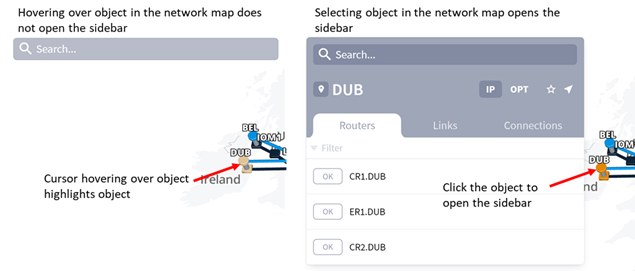
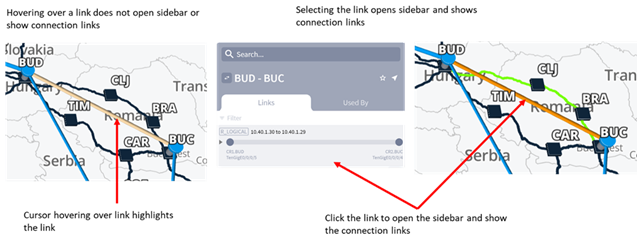
Click an object to view its details in the sidebar (see Sidebar). When you hover your mouse over an object in the network map, the object is highlighted in the map, but no other details are shown. To view details of the object, you must click it to open the sidebar Figure 15). To view a router or a ONE in the network map, hover the mouse over the object (Figure 15). To view a list of routers or ONEs on a site, in the sidebar, click the site to display a list of all the NEs on the site (Figure 15). To view an LSP path, hover the mouse over an LSP link in the network map (Figure 16). To locate an optical connection path, click an LSP path. The connection paths are highlighted in green in the network map and its details are shown in the sidebar (Figure 16). |
| Zoom into a specific area of the map. Note that this process also expands grouped sites to show their objects. |
Use the mouse scroll wheel while in the network map. Press the + (plus) and - (minus) keyboard keys. |
| Center the map on an object. |
Select an object and then click |
| Add object to list of starred objects. |
Select an object and then click |
| View the previous tab in the sidebar. |
When navigating between tabs and objects in the sidebar, click the browser back button to view the previous tab. This is especially useful when you are drilling up or down the layers. |
| Resize the sidebar. |
Resize the sidebar by moving the cursor to the right-hand edge of the window until a double-headed arrow appears. When this arrow appears, click-and-drag it to make the sidebar wider or narrower. This is especially useful in the Paths tab. |
| Scroll down the Paths tab faster. |
In the Paths tab, to scroll down the path faster, click Labels to switch the labels off. |
| Hide layers in Paths tab. |
In the Paths tab, to hide layers, click This applies to all sections in the Paths tab where the composition of the layers is the same.
When the header changes in the Paths tab (that is the composition of the layers changes), you can select to hide the relevant layers in this section (again this applies to all section with the same composition).
You can also deselect all the layers in a section.
|
Examples of Viewing an Object and its Details
Examples of Viewing a Link
The network map models the multilayer, multi-vendor network, including topology, reserved TE-LSP bandwidth, LSP paths, and optical connection paths. This topology includes the crosslinks that connect the network layers, thus enabling you to see the relationship between the IP/MPLS and Optical layers. More specifically, you can see the optical paths that an L3 link or LSP traverses, and conversely see the L3 links that use any given L0/L1 link. You are visually alerted to failures in both layers, as well as given visual cues when reserved TE-LSP bandwidth thresholds are being met.
How often the network map is updated varies, depending on how equipment is configured. Therefore, this update range could differ greatly. For information on how often your model is updated, contact your system administrator or Cisco support representative.
Note: The network map has several controls for changing how it is visualized. You can also show one or both layers in the network map. For information on how to use these network map and site features, see Explorer.
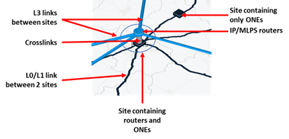
The network map shows the following objects, which consist of sites, links, and crosslinks.
Note: All links and crosslinks are shown in aggregate on the network map.
● Sites contain ONEs (optical network elements), IP/MPLS routers, or both.
● L0/L1 links connect ONEs.
● L3 links connect routers.
● Crosslinks connect ONEs to routers.
Examples of Viewing a Link
The term link applies to both Optical and IP/MPLS layers. All parallel links are visualized as one in the network map. Links are parallel if they are both in the same layer and if their two connecting sites are common. If any one of the links is not available due to failures or other non-operational states, they are shown as red. For more information on IP links and optical links, see IP/MPLS Layer and Multilayer Paths and Optical Layer and Multilayer Paths, respectively.
● Optical links, also known as L0/L1 links, show in the lower layer of the network map. These links also show the connection paths when connections are selected. The L0/L1 link name format identifies the ONE on each end of it, which are colored in black.
<ONE_name>:<port_name> - <ONE_name>:<port_name>
● IP links, also known as L3 links, show in the upper layer of the network map (colored in blue). These links also show the LSP paths when LSPs are selected. The L3 link name format identifies the router on each end of it.
<interface_IP_address> - <interface_IP_address>
Crosslinks show the connectivity between the Optical and IP/MPLS layers. All crosslinks within the site are visualized as one crosslink. For example, if the site contains ONE-A connected to router A and it contains ONE-B connected by two different crosslinks to router B, the crosslink on the network map represents three crosslinks.
The crosslink name format identifies the router and the ONE.
<router_name>:<interface_name> - <ONE_name>:<port_name>
For information on viewing the details of crosslinks, see Multilayer Crosslinks.
| To |
Do This |
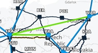
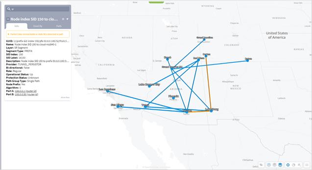
| Show all L3 links that traverse an L0/L1 link |
Select the L0/L1 link. It becomes orange, and all L3 links that traverse the selected L0/L1 link become green. Below is an example of a selected L0/L1 link that is traversed by two L3 links. |
|
|
|
| Show all L0/L1 links over which an L3 link traverses |
Select the L3 link. It becomes orange, and all L0/L1 links that it traverses become green. Below is an example of a selected L3 link that traverses three L0/L1 links. |
|
|
|
Sites typically represent ONEs and routers that are clustered together to represent a small city, region, data center, or a central office. They are positioned on the network map according to their general geographical location. Each site contains one or more ONEs, routers, or both. A site can also include radio devices.
The sites in the network map when it is shown in the default size (not zoomed) can be parent or grouped sites. that contain child sites. You can have many levels of parent/child sites, and child sites can have other child sites. This visualization is configured by the Crosswork Hierarchical Controller administrator.
| If a Site Contains… |
Site Visualization |
| Only routers whether directly or indirectly with nested sites containing only routers. |
|
| Only ONEs whether directly or indirectly with nested sites containing only ONEs. |
|
| At least one router, at least one ONE, and at least one crosslink connecting a router and ONE, whether directly or due to nested sites within it. If a crosslink has not been discovered yet, the site temporarily appears without it. |
|

Expanding and Collapsing Grouped Sites
To expand grouped sites to view their objects or to collapse these grouped sites into one, use the mouse scroll wheel to zoom in or out. Zooming in expands the grouped sites. Zooming out collapses them. Note that zooming in also enlarges the map. To find a specific site, click and hold the map while dragging it to the location of that site. The example below shows a collapsed grouped site and its expanded view.
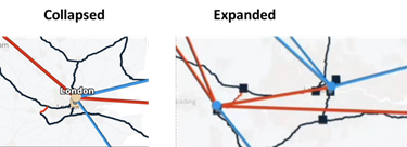
Expanded Site
| Link |
Description |
| Fiber segment |
Physical fiber line that spans from one passive fiber endpoint (manhole, splice etc.) to another and is used as a segment in a fiber link. |
| Fiber |
Chain of fiber segments that spans from one optical device to another. |
| OTS |
OTS is the physical link connecting one line amplifier or ROADM to another. An OTS can be created over a fiber link. |
| OMS |
OMS is the link connecting between one ROADM and another. An OMS can be created over a chain of OTS links. |
| NMC (OCH-NC, OTSiMC) |
NMC is the link between the xPonder facing ports on two ROADMs. This link is the underlay for OCH and it is an overlay on top of OMS links. This is relevant only for disaggregation cases where the ROADM and OT box are separated. |
| OCH |
OCH is a wavelength connection spanning between the client port one OT device (transponder, muxponder, regen) and another. 40 or 80 OCH links can be created on top of OMS links. The client port can be a TDM or ETH port. |
| SCH |
A super-channel is an evolution of DWDM in which multiple, coherent optical carriers are combined to create a unified channel of a higher data rate, and which is brought into service in a single operational cycle. |
| STS |
Large and concatenated TDM circuit frame (such as STS-3c) into which ATM cells, IP packets, or Ethernet frames are placed. Rides on top of OC/OCG as optical carrier transmission rates. |
| OC/OCG |
SONET/SDH links that span from one optical device to another and carry SONET/SDH lower bandwidth services, the links ride on top of OCH links and terminate in TDM client ports. |
| ZR Media |
The media layer as a carrier of ZR channels, on top of OCH link. |
| ZR Channel |
Multiple ZR channels can be on top of ZR media, each channel represents a different IP link with its own rate. |
| Radio Media |
The media layer as a carrier of radio channels. |
| Radio Channel |
Multiple radio channels can be on top of radio media, each channel represents a different ETH link with its own rate. |
| OTU |
OTU is the underlay link in OTN layer, used for ODU links. It can ride on top of an OCH. |
| ODU |
ODU links are sub-signals in OTU links. Each OTU links can carry multiple ODU links, and ODU links can be divided into finer granularity ODU links recursively. |
| ETH link |
ETH L2 link, spans from one ETH UNI port of an optical device to another, and rides on top of ODU. |
| ETH chain |
A link whose path is a chain of Ethernet links cross-subnet-connected (found using Crosswork Hierarchical Controller cross-mapping algorithm). Eth-chain is a replacement for R_PHYSICAL link in cases where one side of the link is in devices out of the scope discovered by Crosswork Hierarchical Controller. |
| L3 physical |
L3 physical is the physical link connecting two router ports. It may ride on top of an ETH link if the IP link is carried over the optical layer. |
| Agg link |
Agg is Link Aggregation Group (LAG) where multiple ETH links are grouped to create higher bandwidth and resilient link. |
| Logical link, IGP, LSP |
Logical link connects VLANs on two IP ports. |
| IGP |
IGP is the link between two routers that carries IGP protocol messages. The link represents an IGP adjacency. |
| LSP |
LSP is the MPLS tunnel created between two routers over IGP links, with or without TE options. |
| SR Policy |
A segment routing path between two nodes, with mapping to the IGP links based on SIDs list |
| L3-VPN link |
The connection between two sites of a specific L3-VPN (can be a chain of LSP connections or IGP path). |
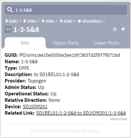
Each crosslink represents an L3 interface connection to an L0/L1 port. Studying crosslinks and multilayer paths (where and how routers connect to ONEs [optical network elements]) gives you an understanding of how network traffic is flowing. Knowledge of this port mapping between the two layers is essential for identifying how taking down an optical link will affect the network at both layers. This information is also useful, for instance, when optimizing the network and configuring it for restoration.
Exploring Multilayer Crosslinks
The network map shows these crosslinks in aggregate. For example, Figure 18 shows a router in a data center connected to a ONE using 3 crosslinks. These three crosslinks appear in the network map as one. Selecting the site enables you to determine how many interface-to-port mappings there are per site, and enables you to drill down to the details of each individual crosslink in the sidebar (Figure 19). To view details of a crosslink, you must click on the column of the crosslink that connects the L0/L1 layers to the L3 layer.
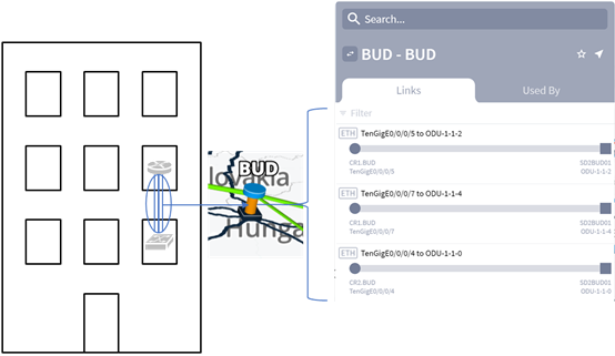
Discovered and Visualized Crosslinks
The crosslink name format identifies the router and the ONE.
<router_name>:<interface_name> to <ONE_name>:<port_name>
Example: Figure 19 shows that the L3 interface E0/0/0/5 on the CR1.BUD router is connected to the L0/L1 port 1-1-2 on the SD2BUD01 ONE.
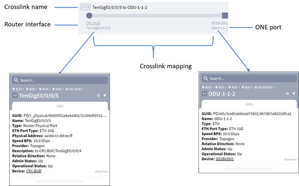
Example Crosslink
IP/MPLS Layer and Multilayer Paths
The 3D Explorer UI enables you to explore the IP/MPLS layer and its relationship with the Optical layer. As outlined in Network Map, the network map sites containing routers represent all routers within the site as one. L3 links between sites are all represented as one link.
This topic describes how to further explore the IP/MPLS layer and its relationship with the Optical layer beyond what is in the network map and site views. Understanding this multilayer relationship helps you better plan the L3 topology and route L3 traffic. For instance, by exploring IP/MPLS and multilayer features you might find that L3 links or LSPs share risk of failure at the Optical layer because they share optical links. You might find that the LSP path hops are not optimized for the best routes.
To view details about the IP/MPLS layer, select a site containing a router from the network map. A sidebar opens to the IP tab. From here you can explore details on routers, L3 links, ports, LSPs, and multilayer paths by clicking on any of the sub-tab that appear. Available sub-tabs are listed below. Some sub-tabs may not be visible, depending on what is selected.
● Routers—All routers within the site or a selected router. You can view the details of a router at the site by clicking it in the sidebar, see Exploring Routers.
● Ports—All logical and physical ports on the selected router.
● Links—If a site is selected, these are all L3 links to routers within the site. If a router is selected, these are all the L3 links connected to it. If an L3 link is selected, these are all L3 links between the sites on either end of the selected link. This list includes link bundles, also known as aggregated links, port bundles, or LAGs. (A link bundle is a logical grouping of physical interfaces so that they can be easily configured and maintained as one.)
● Used By—Shows all links and connections that are in the layer above the displayed link/connection.
● Connections—If a site is selected, these are all LSPs going through all routers in the site, regardless of whether the router is a source, a destination, or a hop (transit router). If a router is selected, these are all LSPs going through that router. If an L3 link is selected, these are all LSPs traversing that link.
● Paths—Describes the path of the selected element. The LSP path shows each hop (source, destination, and transit) used by the LSP. If a site is selected, these are LSP paths going through all routers in the site. To view the LSP path, click the LSP name. If a router is selected, these are all LSP paths traversing all L3 links connected to that router. If an L3 link is selected, these are all LSP paths traversing that link. The optical path for the L3 links that are traversed is also shown.
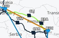
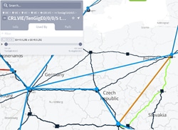
Selecting any L3 link in the network map highlights it in orange and highlights the L0/L1 links and connections that the L3 object traverses in green. For example, Figure 21 shows a selected L3 link between CR1.VIE and VR2.WAR uses three L0/L1 links.
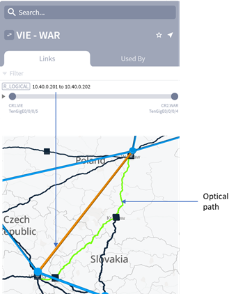
Selecting an L3 Link Highlights Its L0/L1 Path
Selecting a site containing routers opens a sidebar that shows all routers in the site.
Sidebar Showing Routers at Site
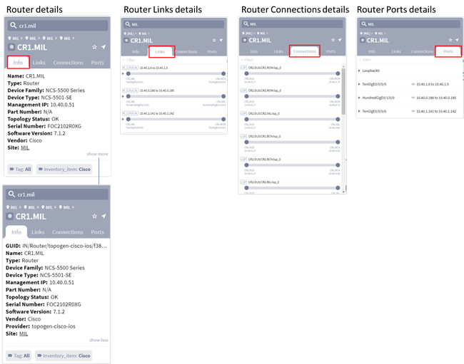
Example of a Site in the Sidebar Showing the Routers, Links, Connections and Ports
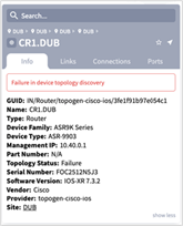
Example of an Unreachable Router
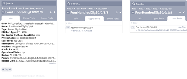
Example of Port Info, Upper Ports and Lower Ports
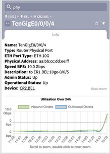
Example of Router Physical Port Utilization
To view details about a router, select it. The sidebar shows the following details for the selected router:
● Info: Shows information about the router, including its GUID, name, type, device family, device type, management IP, part number, topology status, serial number, software version, vendor, provider, and site. Click show more or show less to see more or fewer details. If a device is unreachable a message appears. For an example, see Figure 24.
● Links: Lists the router’s logical interfaces. Click the arrow to see the physical interfaces.
◦ If the space on the right is empty, the L3 link or crosslink is unknown.
◦ If the crosslink to the ONE is known, the expansion shows the router’s physical interfaces and the ONE’s ports, as well as a crosslink icon.
● Connections: Lists the router’s LSP connections.
● Ports: Lists the router’s ports and the links connected to each port. The Admin Status (Up or Down) and the Operational Status (Up or Down) can be viewed when drilling down on a port to the Info tab.
Note: You cannot view all ports for a site. You can only view them on a per-router basis.
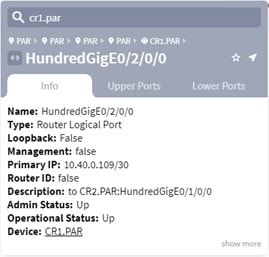
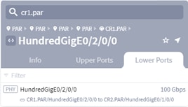
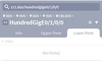
To view details about a router physical or logical port, select it. The sidebar shows the following details for the selected port:
● Info: Shows information about the physical or logical port. For a physical port, its GUID, name, type, physical address, speed, provider, admin status, operational status, relative direction and device. For a logical port, its GUID, name, type, loopback, stats dummy, provider, admin status, operational status, relative direction, device and relative port. Click show more or show less to see more or fewer details. If the router is tagged, the tags appear at the bottom of the tab.
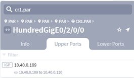
● Upper Ports: Lists the upper ports. The upper port details appear when drilling down on a port.
● Lower Ports: Lists the lower ports. The lower port details appear when drilling down on a port.
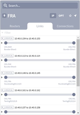
The blue lines connecting sites on the network map indicate the L3 links between sites. However, as there may be numerous L3 links between sites, they are not all shown in the network map. Consequently, the blue line between sites also represents the sitelink between two sites. Click on a link in the map to show its details (Figure 27).
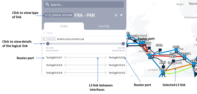
Example showing Sidebar with Details of Logical Sitelink Selected in the Network Map
Note: Connections shown in red indicate that the connections are down.
The Links tab in the sidebar shows the following information (Figure 27):
● Type of link—In this example, a logical sitelink that indicates the names of the connected sites.
● L3 link name—The name of the link named according to the IP addresses at each end of the link in the form:
<interface_IP_address> to <interface_IP_address>
All links appear with a clickable arrow pointing to the link name, indicating that you can expand the link to show the names of the respective ports on each end of the link within it (Figure 27).
To view details of the logical link, click the link name in the Links tab (Figure 27). The sidebar now shows details of the L3 link including the names of the logical and physical ports at each end of the link, as well as the link itself. The Info tab also shows more details of the link as shown in Figure 28.
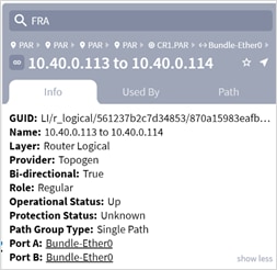
Sidebar Showing Logical Link
If an L3 link is not available due to failures or other non-operational states, it is shown as red in the network map. L3 links are marked as Down in the sidebar if a router on either end of the link does not identify the logical interface in the ARP table. To view details on any of the logical or physical ports, click on the port link in the sidebar.
Example of Logical Port Info, Upper Ports and Lower Ports
You can also view logical links in a site by clicking the site and then selecting the Links tab in the sidebar.
Example of the Links in a Site
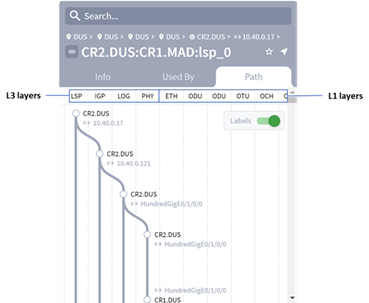
In the sidebar for a logical link, click the Path tab to the visual details of all the layers in the logical link including the L3 and L1 layers.
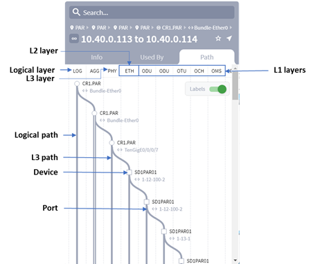
Example of the Layers in a Path of a Logical Link.
Note: The above example shows the layers in a logical link. These layers may differ according to the links used in your network and according to the level at which you viewed the paths. For example, in Figure 31, the path was viewed from the logical layer. If the path was viewed from the physical layer level, the path of the logical layer does not appear. This means that the paths shown are always the paths downwards from the level from which you view the path.
Figure 32 shows an example of the layers in a path from the LSP level downwards. For more information on LSPs, see Exploring LSPs.
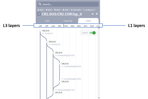
Example of LSP Path Layers
You can configure an aggregate interface on a router. This adds another layer to the path. Figure 33 is an example of an aggregated link between two routers.
Aggregate Links between Two Routers
Link bundles show as parallel L3 links (Figure 34).
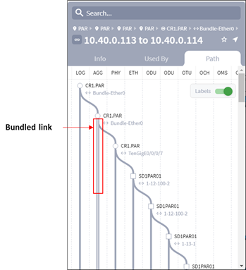
Bundled Link in Path Tab
Clicking the area to the right of the aggregated link, changes the selected link sequentially up (to the right) or down (to the left). Each time you click to show a new L3 link, the optical path changes to reflect the newly selected L3 link).
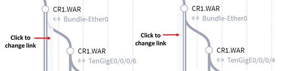
Selecting Links in Bundled Link in Path Tab
The sidebar lists the LSPs traversing or using the currently selected object in the network map. For example:
● If a site is selected, the Connections tab in the sidebar lists all the LSPs starting and ending at the site.
● If a link between sites is selected, drill down until a logical link is selected. The Used By tab in the sidebar lists all the LSPs traversing that link.
Exploring L0/L1 Paths Traversed by LSPs
To locate an LSP, click on a site in the map to show its details in the sidebar. Then click the Connections tab to view all the LSP links that traverse the site (Figure 36).
Connections Tab showing LSP Links
Clicking the LSP name in the sidebar shows you both the LSP paths and the optical paths it traverses in the network map. At the same time the sidebar changes to show the Info, Used By and Path tabs for the selected LSP. The LSP paths are shown in orange, while optical links it traverses are shown in green (Figure 37).
LSP and Physical Links
When expanded, an LSP shows the following information:
● LSP path
◦ Source site or source router—LSP head end.
◦ Destination site or destination router—LSP tail end.
● LSP name
● LSP path showing the hops that the path takes
● In the network map, the logical and optical paths are highlighted in orange and green respectively
Click the Path tab to view the LSP path details.
LSP Path Details
Click on a router name in the Path tab to view its details. Likewise you can click on a port name in the Path tab to view its details (Figure 39).
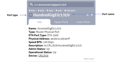
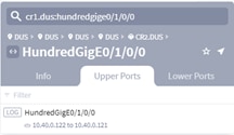
Port Info Tab & Upper Ports & Lower Ports
Click on any of the vertical path lines in the Path tab (Figure 38) to view its details in the respective Info, Used By and Path tabs for that path.
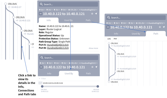
Path Details
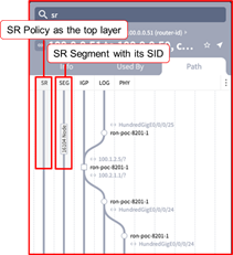
The network model supports Segment Routing (SR) Policies. An SR Policy is modelled as a tunnel comprising multiple SR Segments over IGP links.
Each SR Segment is a link in the model represented by a SID, that is configured in the end node of the SR Segment. For example, the first SR Segment in the example below is between A and the node configured as SID C. The second SR Segment is between C and the node configured as SID B.
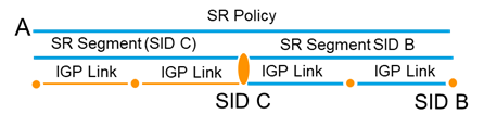
SR Policy
A SID can be associated with multiple SR Segments with different starting points (and the same endpoint based on the SID), and can also be used in multiple SR Policies.
Crosswork Hierarchical Controller adapters can discover policies from network controllers, with their SID list, color, preference, and candidate path attributes. It maps all discovered policies to create SR Segments as a layer between IGP links and SR policies. An SR Segment is the path between two SIDs, shared by multiple SR policies.
In addition, SR Segment routing configuration is modelled for the device, card and IGP interface.
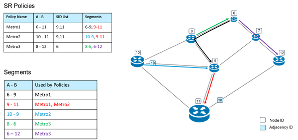
SR Policies and Segments
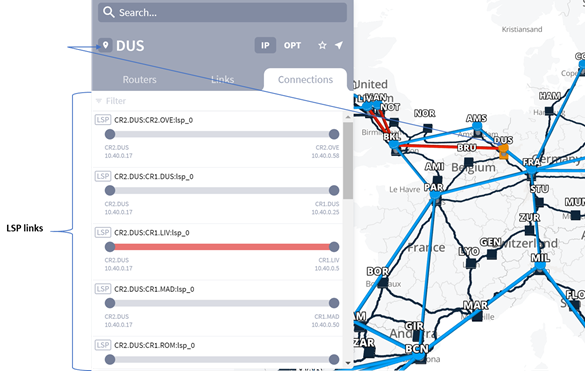
To view a list of SR Policies, select the Network Inventory application and then click on the Connections tab.
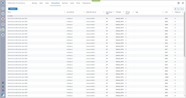
SR Policies in Network Inventory
The network map shows you a visual representation of the SR Policy and the SR Segments over IGP links. Selecting any SR Policy in the network map highlights the links in the color is specified when the policy is provisioned using the Service Manager application.
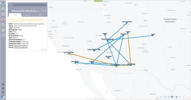
SR Policies and SR Segments
Click on the Path tab to view the path of the current SR Policy including the SR Segments over IGP links.
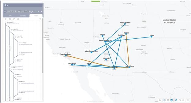
SR Policy Path
SR Policy Path
Select an SR Segment to view it’s path between two SIDs.
SR Segment
An SR Segment may be shared by multiple SR policies. To view the SR Policies above the selected element, select the Used By tab.
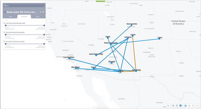
SR Segment Used By
Optical Layer and Multilayer Paths
The 3DExplorer UI enables you to explore the Optical layer and its relationship with the IP/MPLS layer. As outlined in Network Map, sites in the network map containing ONEs (optical network elements) represent all ONEs within the site as a single ONE icon. L0/L1 links between sites are all represented as one link. To drill down into the site to explore its ONEs and their intrasite relationships, double click on a site in the network map.
This topic describes how to further explore the Optical layer beyond what is in the network map and site views.
Note: To view multilayer paths in the sidebar, see IP/MPLS Layer and Multilayer Paths.
To view details about the Optical layer, select a site containing a ONE from the network map. A sidebar opens to the IP/MPLS tab. From here, select the OPT tab so you can explore details on ONEs, L0/L1 links, ports, and connections by clicking on any of the tabs that appear. The following tabs are available, although they may or may not be visible, depending on what is selected.
Note: If you select a site in the network map that only contains ONEs, the OPT link is automatically opened.
● Nodes—All ONEs within the site or a selected ONE.
● Info—Details about the node. If the node is tagged, the tags appear at the bottom of the tab.
● Links—If a site is selected, these are all L0/L1 links to and from ONEs within the site. If a ONE is selected, these are all the L0/L1 links connected to it. If an L0/L1 link is selected, these are all L0/L1 links between the sites on either end of the selected link.
● Ports—All physical ports on the selected ONE.
● Connections—If a site is selected, these are all connections going through all ONEs in the site, regardless of the positions of the ONEs in the path. If a ONE node is selected, these are all connections going through that ONE node.
● Used By—Shows all links and connections that are in the layer above the displayed link/connection.
● Paths—Describes the path of the selected element.
Selecting any L0/L1 object in the sidebar highlights it in the network map as orange.
Exploring ONEs and their Ports
Selecting a site containing ONEs opens a sidebar that shows all ONEs in the site. To view details about a ONE, select it.
To view optical ports, select a ONE from the sidebar and then select the Ports tab. For an example, see Figure 50.
● The L0/L1 port type is labeled as ETH, ODU, OTU, OCH, OMS, OTS, FIBER, or FSEG.
● The ODU ports are further labelled by type.
Note: You cannot view all ports for a site. You can only view them on a per-ONE basis.
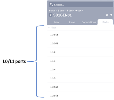
Example Ports Tile Showing Ports Used by L0/L1 Links and Crosslinks
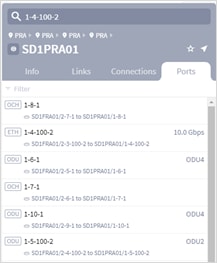
Example ODU Port Types
Note: If a port is down is appears in red in the Ports tab.
Click a port to view its details in the Info tab. The port view includes the Upper Ports tab and Lower Ports tab.
Port Info Tab
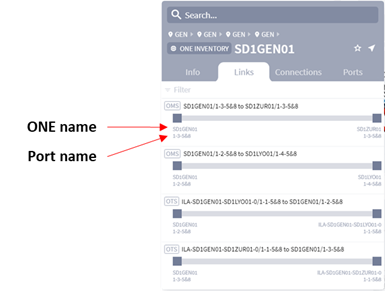
The L0/L1 link name format identifies the ONE on each end of it.
<ONE_name>:<port_name> to <ONE_name>:<port_name>
Links show the ONE name, and port name (Figure 51). If an L0/L1 link is not available due to failures or other non-operational states, it is shown as red in the network map. L0/L1 links are marked as DOWN in the sidebar if the controller or management system identifies it as down.
Example L0/L1 Link
Exploring L3 Links that Traverse L0/L1 Links
The network map shows you a visual representation of the relationship between the Optical and IP/MPLS layers. However, the network map representation is of all links going between the two sites. The sidebar enables you to view these relationships on a per-L0/L1 link basis.
Selecting any L0/L1 link in the network map highlights the L3 links that use the L0/L1 link in green.
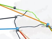
Example: Figure 53 shows a selected L0/L1 link between BRAT and KRA has two L3 links traversing it.
Selecting an L0/L1 Link Highlights the L3 Links Traversing It
To view the elements in the layers above the selected element, select the Used By tab and select the required element. Click on the Path tab to view the path of the current element.
Repeat to step through the elements in the layers above the selected element. The map is updated as you navigate through the elements.
Navigating Layers
You can continue viewing the elements in the layer above until there are no elements in the Used by tab.
LSP
The 3D Explorer UI enables you to locate radio devices of type:
● Indoor_Unit (IDU)
● Outdoor_Unit (ODU)
● Radio_Antennae
● All_Outdoor_Unit (an all-in-one radio device).
When you select a radio device in 3D Explorer, the site is highlighted.
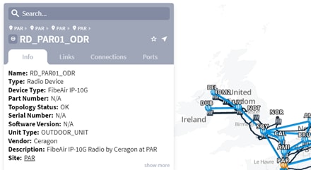
Radio Device
A radio channel (Routeradio Channel) represents the physical radio layer of a microwave network. Radio-channel ports model “radio” endpoints of the radio-side network (as opposed to client-side ports that serve as end-points of client services such as Ethernet, SONET/SDH, and PDH).
Radio-channel ports are physically connected to radio outdoor units (ODUs) and from there to antennas. These ports contain rf-physical-parameters such as modulation, frequencies, bandwidth, and power, in addition to regular port fields.
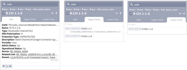
Radio Channel
Between two radio-channel ports having radio-connectivity there is a radio-channel link (link with layer ‘radio-channel’).
Note: The radio-channels links are not currently represented on the 3D Explorer map.
Since a single radio-channel has limited capacity, many vendors have some sort of proprietary mechanism for aggregating multiple radio-channels between same sites into a single managed entity having the sum capacity of the radio links below it (different vendors have different names for this aggregation, but it is essentially very similar).
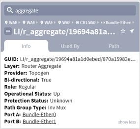
This aggregation (Routeradio Aggregate) is modelled in Crosswork Hierarchical Controller as a RadioAggregate link. By having this aggregation onthe radio-side, vendors allow a more robust use of the total capacity as this capacity can be used “elastically” to transport higher capacity client services that cannot fit in a single radio-channel, or transport multiple smaller capacity services while optimally using the radio-bandwidth.
This aggregation can also be used as a form of protection when the available aggregated capacity is bigger than the needed capacity, allowing the network to pass traffic using active radio-links if some become inactive, or if the total capacity is reduced because of weather conditions.
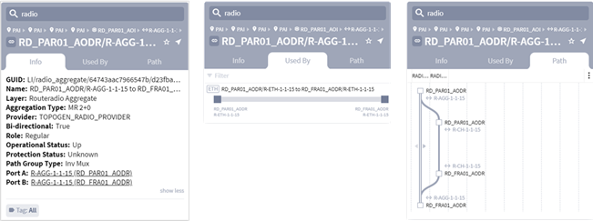
Radio Aggregate
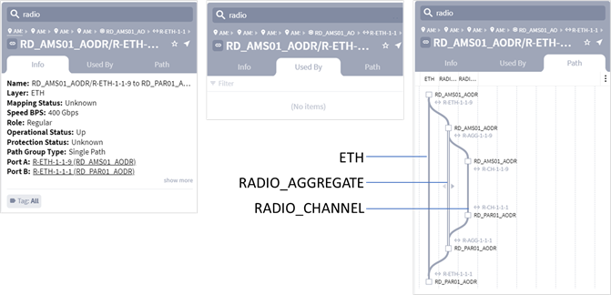
ETH Layer powerd by Radio
The time machine provides a snapshot of the state of the network as it was at a date in the past. In this mode, all applications reflect data and analysis that apply to this point in time.
The applications that support time machine are:
● 3D Explorer
● SHQL Dashboard
● Network Vulnerability
● Network Inventory
● Path Optimization
● Failure Impact
● Shared Risk Analysis
● RCA
● Services Manager (without configuring new services)
Click Live, select a date and click Confirm.

Time Machine
You are now viewing the network as at the selected date. Click Back to Live to return to return to the current view of the network.
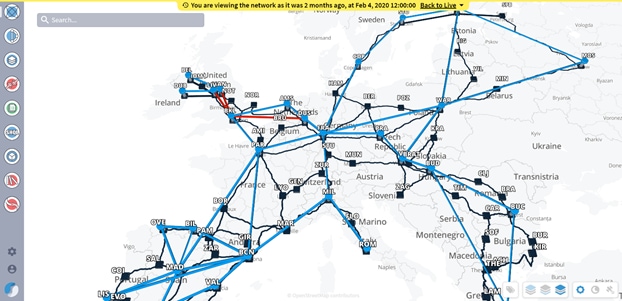
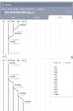
Explorer with Time Machine Applied
The Layer Relations application enables you to see the relationship between the different layers in the network. Navigation up and down the layers of the network enables you to better understand how the network is structured.
Within the application a layer can be designated as a Primary Object or a Related Object. These terms are used for comparison purposes only and should not be interpreted as meaning that a Primary Object is higher in the layer hierarchy than the Related Object, and vice versa.
The purpose of the applications is therefore to show the relationship between two selected layers. This means that you can select any layer as a Primary Object and any layer as a Related Object, no matter where they appear in the hierarchy, and you can inverse between them. For example, if you select your Primary Object as L3 Physical and the Related Object is OMS, you are shown a list of all the L3 Physical links and the OMSs they are using.
The Layer Relations application enables you to compare the following layer types in a network.
● LSP
● SR Policy
● SR Segment
● IGP
● L3 Logical
● L3 Physical
● L3 Aggregate
● Ethernet Chain
● Ethernet
● ODU
● OTU
● OCH
● NMC
● OMS
● OTS
● STS
● STS Virtual Group
● OCG
● OTN
● Fiber
● Fiber Segment
● Radion Channel
● Radio Aggregate
● Radio Medium
● ZR Channel
● ZR Media
Using the Layer Relations Application
You access the Layer Relations application by clicking the Layer Relations icon on the left of 3D Explorer network map.
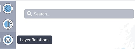
Layer Relations Application
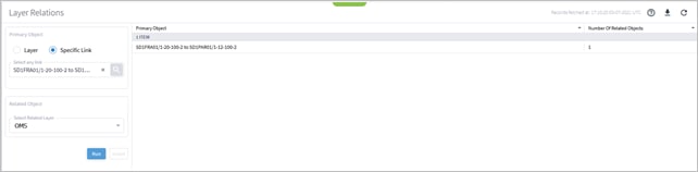
The Layer Relations user interface opens as follows: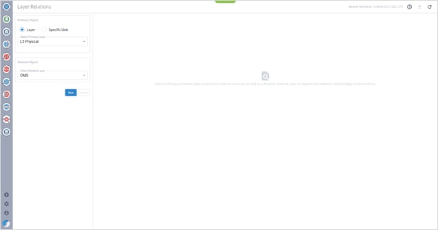
Layer Relations User Interface
You can choose to view the layer relations between layers or between a specific link and layers within that link.
Note: If a Related Object does not exist for the selected Primary Object, no results are shown, even if there are other layers in the Primary Object. For example, if you select L3 Physical as your Primary Object, and want to see the related OMS links. If there are no OMS links, no results are shown even though there may be OTS links related to the Primary Object.
Viewing Layer Relations Between a Specific Link and a Layer
You can view relations between layers where the Primary Object is a Layer or the Primary Object is a Specific Link. This topic describes how to view layer relations where the Primary Object is a specific link. For information on how to view layer relations where the Primary Object is a layer, see Viewing Layer Relations Between Layers.
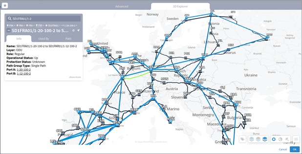
This example shows the layer relations when you choose a specific link as the Primary Object and OMS as the Related Object. Bear in mind that you can choose any link as the Primary Object and any layer as the Related Object irrespective of where they are in the hierarchy.
To view layer relations between a link and a layer:
1. Select the Specific Link option.
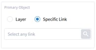
2. Click to select a link.
3. Select a link in the Advanced tab or in the 3D Explorer to select a specific link as your Primary Object.
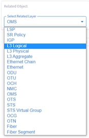
4. In the Related Object area, from the Select Related Layer Type dropdown list, select the related layer type.
The following image shows the selected Primary and Related objects.
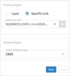
5. Click Run.
A list of Primary Objects that match your selection is generated and appears on the right side of the screen.
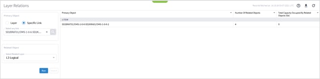
View details and information about the links as described in Viewing Layer Relations Between Layers.
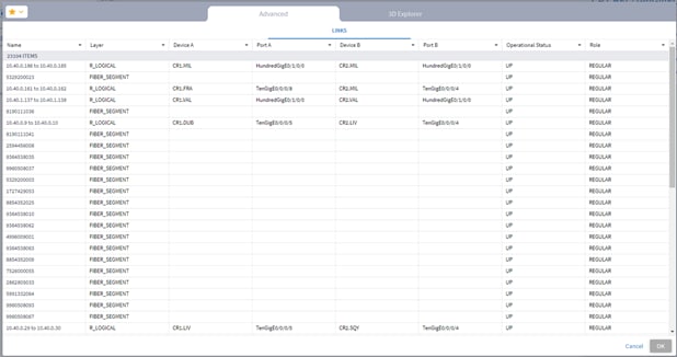
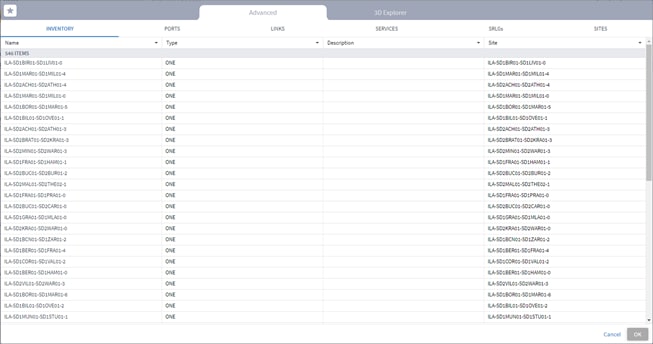
The Model Selector is a tool used to select objects. It lists details of the links and ports in the network and enables you to filter the list according to your requirements.
This topic describes how to use the Model Selector for selecting a specific link for which you want to find Related Objects in the network.
To select a specific link using the Model Selector:
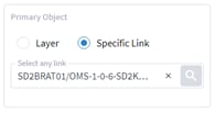
1. In the Primary Object area, select the Specific Link option.
The Find box appears.
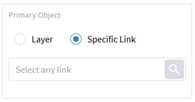
2. Click the Find icon.
The Model Selector window opens.
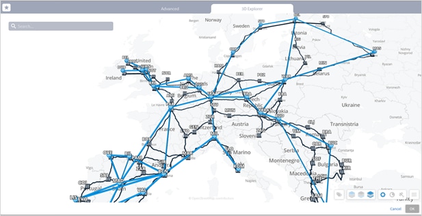
3. Find and select a link in the 3D Explorer.
4. Click OK.
5. Click Run. The link with its related objects appears.
6. Alternatively, click the Find icon.
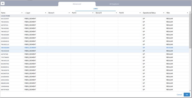
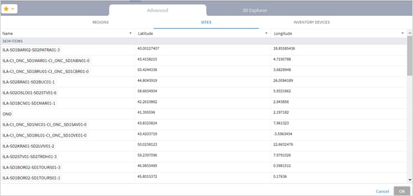
7. Click the Advanced tab.
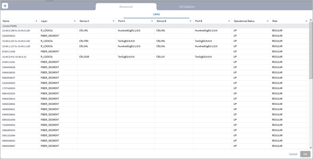
8. Click a column heading to sort the column in ascending or descending order.
9. To filter a column, click the Filter icon to the right of the column heading and enter the filter criteria in the Filter box.
10. Click a link to select it or click and select a starred item.

11. Click OK to accept your selection and return to the Layer Relation page.
Viewing Layer Relations Between Layers
You can view relations between layers where the Primary Object is a Layer or the Primary Object is a Specific Link. This section describes how to view layer relations where the Primary Object is a layer. For information on how to view layer relations where the Primary Object is a specific link, see Viewing Layer Relations Between a Specific Link and a Layer.
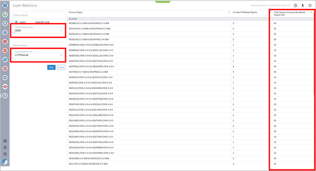
This example shows the layer relations when you choose L3 Physical as the Primary Object and OMS as the Related Object. Bear in mind that you can choose any layer as the Primary Object and any layer as the Related Object irrespective of where they are in the hierarchy.
To view layer relations between layers:
1. Select Layer.
2. In the Primary Object area, from the Select Primary Layer dropdown list, select the primary layer type.
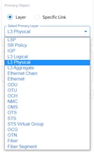
3. In the Related Object area, from the Select Related Layer Type dropdown list, select the related layer type.
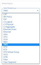
The following image shows the selected Primary and Related objects.
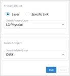
4. Click Run.
A list of Primary Objects that match your selection is generated and appears on the right side of the screen.
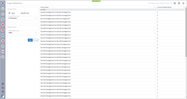
The Primary Objects area lists links to all the primary objects that meet your selection (in this case L3 Physical links) and indicates the Number of Related Objects in a column on the right of the screen.
The link L3 link name format identifies the ONE on each end of it, in the format:
<ONE_name>:<port_name> - <ONE_name>:<port_name>
Note: The Inverse button is activated at this time. This enables you to show the inverse relations between the selected layers. In this example if you click Inverse, OMS becomes the Primart Layer Type and L3 Physical becomes the Related Layer Type. Click Inverse again to go back to your initial selection.
If the Primary Object is lower in the hierarchy than the Related Object, an additional column on the right shows the Total Capacity Occupied by the Related Objects, as shown in the following example.
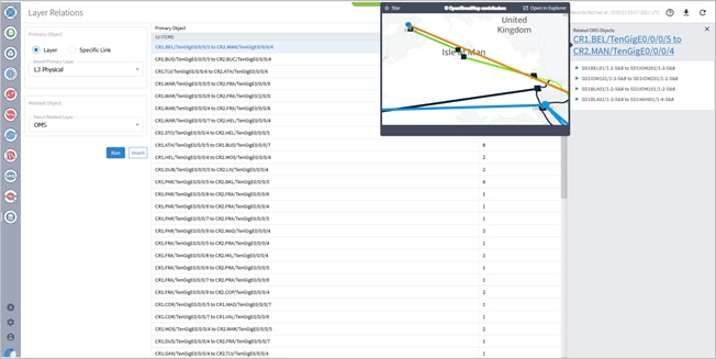
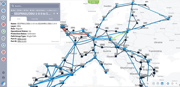
5. Click on a Primary Object to display the related objects and then hover over the link in the Related Objects pane. The network map appears with the hovered link in orange.
6. Click to expand the related links (in this example, the related OMS links).
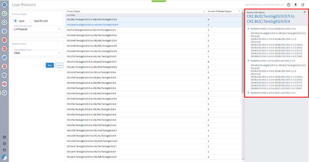
The related link name format identifies the ONE on each end of it, and the ports to which they are connected in the format:
<ONE_name>:<port_name> - <ONE_name>:<port_name>
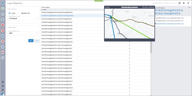
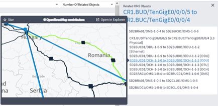
7. Hover your cursor over a Related Object link to display the section of the network map where the hovered link appears. The hovered link appears in orange in the network map.
8. Click on the arrow of a Related Object link to view the path of the Primary Object link and the paths of all the layers that are related to the Primary Object link, including the selected Related Layer (in this case the OMS layer).
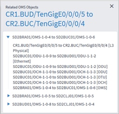
The related link name format identifies the ONE on each end of it, and the ports to which they are connected in the format, and includes the name of the layer:
<ONE_name>:<port_name> - <ONE_name>:<port_name>[layer_name]
9. Hover your cursor over a Related Object link to display the section of the network map where the hovered link appears. The hovered link appears in orange in the network map.
10. Click a link in the list to drill down to the link in Explorer.
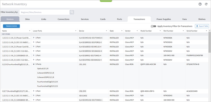
The Network Inventory app shows a full tabular view of devices, sites, links, connections, services, cards, ports, transceivers, power supplies, fans, and shelves.
The purpose of this application is to allow users to explore, in a filterable and sortable table format, the various resources that Crosswork Hierarchical Controller maintains and which constitute their network.
The data is broadly categorized as follows:
● Devices (Routers, Optical Network Elements, Radio Devices)
● Sites
● Links (Fiber, Radio Channels, Radio Aggregates, OTS, OMS, ZR Media, ZR Channel, L3 Physical, L3 Aggregate, L3 Logical, IGP, SR Segment, MC)
● Connections (NMC, OCH, OUT, ODU, Ethernet, MPLS TP, Pseudo Wire, SR Policy, LSP, MC)
● Services (L3-VPN, E-Line, OTN Line)
● Cards (pluggable cards of optical devices and routers)
● Ports (Radio Medium, OTS, ZR Media, ZR Channel, Ethernet, L3 physical (on routers), MC)
● Transceivers
● Power Supplies
● Fans
Resources in each category are organized in tables, are sortable and filterable. Several data analysis tasks are simplified. For example, finding IP links whose metrics are above some specified threshold can easily be accomplished by navigating to the Links tab, choosing IGP links, and applying a greater than (>) filter to the Metric column.
The output will show a list of all links that match the criteria, along with the key attributes of those links (IGP interface, Metric, Router, etc.).
Hovering over cells that correspond to a network entity allows the user to quickly visualize that entity in the context of the network. Clicking on an entity takes the user to the Explorer-based view of that entity.
The tabular data can be exported into a CSV file for offline analysis.
To filter inventory:
1. Click ![]() .
.
![]()
2. In the Advanced tab, select REGIONS, SITES or INVENTORY DEVICES, and select the required item.
Or select the 3D Explorer tab and select the required item.
3. Click OK.
4. Use the Apply Inventory Filter on Devices toggle to view the table with or without the filter applied.
![]()
5. Select the required types, for example, in the Links tab, for example select L3 PHYSICAL.

6. To futher filter any of the result tables, filter using the columns.
To export inventory:
1. Select the required tab and filter the table.
2. Click Export Table. The data is exported to a csv file.
Crosswork Hierarchical Controller models pluggable transceivers as inventory ports with transceiver details as attributes. For cases with multiple ports on the same transceiver, the transceiver details are mapped to the parent inventory port and the sub ports are defined as ‘not pluggable’. The Network Inventory app shows the router physical ports (built on top of the sub ports, which are also inventory ports) as mapped to the transceiver in the Transceivers tab. Click to expand the ports.
The SHQL Dashboard is made up of table, pie or chart widgets. The information presented in a widget is updated periodically, typically every few minutes. The widget includes up to five fields, and 100 items.
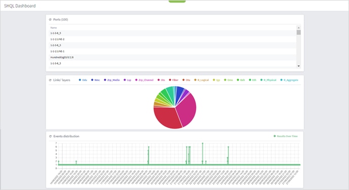
You can create customized widgets, rapidly with no development efforts and no software delivery. The widget query runs when opening the SHQL Dashboard application and the widgets are displayed. The widget also has a refresh button to run the query manually.
The widget attributes are:
● Title: The name of the SHQL widget as it appears in the SHQL Dashboard.
● Query: Must be up to 5 views, and limit(100)
● Visual mode:
◦ Pie/bar – when the query contains counters only
◦ Graph – when the query contains timestamp and counters
◦ Table – when the query returns a list
● ‘About’ text
● Optional: Additional query to be used as a drill down into a widget (can be automatically generated (removing the counter and limit).
1. In the applications bar in Crosswork Hierarchical Controller, select SHQL Widgets.
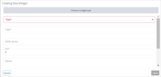
Creating New Widget
3. Select the Type. This can be Table, Graph, or Pie.
Depending on the type of widget selected, guidance is provided on the SHQL permitted.
Cisco Crosswork Hierarchical Controller keeps records of all changes in the network inventory and topology. Changes are stored as:
● Snapshots of the network model at different times (used in the Explorer Time machine).
● A list of events (used in the Network History application).
An event is a record of any resource addition, deletion, or attribute change. The event record includes all changes that may potentially help with failure analysis, capacity planning, early detection of outages, and more.
The Network History application enables you to view the events table with all the details of the change including the time, resource ID, object type, event type, and the value before and after the change. You can run queries based on a time range, specific resources (selected by tags, SHQL query or specific resources), event types and by attribute values. Queries can be saved for later use.
A unique implementation was selected to include all resources that were in the model at some point in the selected time range in the returned results. Thus, it guarantees that services or links that were subsequently deleted are still found.
For example, if you filter the table to get events for all services with specific tags for the past two weeks, the results will include the relevant services, including those that no longer exist at the end of the period.
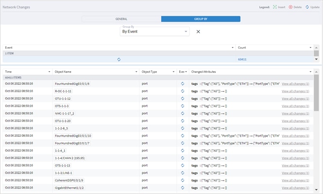
The results are displayed in a table, with options to sort and filter the columns, group by time, object type or event type to get a count of the events.
The Network History application records all changes in inventory, topology, performance, configuration, and status and save them as events. Update, insert and delete events are saved.
The Network History application helps you analyze these events and answer questions, helping you to find correlations between changes such as:
● Discovering that the ports went down after a SW upgrade.
● Noting that the cards reset led to configuration changes.
● Seeing that the outage of certain devices caused rerouting and traffic congestion.
The following changes are recorded.
Inventory:
● New inventory – card, chassis, transceiver
● Card replacement
● SW upgrade
Status:
● Link failures
● Device reachability
● Link and port operation state
● Link and tunnel path rerouted
● VPN site down
Configuration:
● Link and tunnel configuration (BW, admin state, affinities)
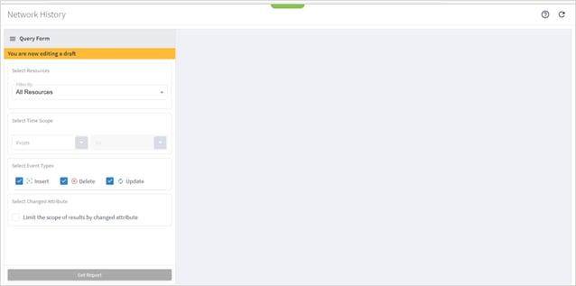
You can complete the query form and then save the query as a network history report. Saved reports are available to all users.
You can select which resources to get the history report for:
● All resources
● By SHQL Query
● By tags
● By specific resources
You can also specify whether you want to query all events or events of a specific type (Insert, Delete and Update). You must also specify a time period. By default, the events for the past 2 days appear.
● In addition, you can limit the scope of results by changed attribute for the following object types:
● Inventory Item
● Link
● Path
● Port
● Region
● Service
● Service Intent
● Service Intent Resource
● Site
● Site Link
● Srlg
● Srlg Risk Resource Mtm
● Visual Site
Note: For more details on the object types and a list of their attributes, see the Cisco Crosswork Hierarchical Controller NBI Reference Guide.
To create a network history report:
1. In the applications bar, select Network History. Alternatively, if you are already in the Network History application, click ![]() New Form.
New Form.
2. To query events for all resources, select All Resources.
3. To query events by SHQL query, select By SHQL Query and then enter an SHQL query. For more information, see the SHQL User Manual.
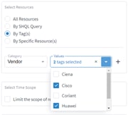
4. To query events by tags, select By Tag(s), and then select a Category and the required Values. Use the + button to add the selected tags.
5. To query by specific resources, select By Specific Resource(s), click to Select Resource and then select the required resource and click OK. You can add multiple items, however, if you want to add many resources, it is recommended to use SHQL or tags.
6. To select specific event types, select Limit the scope of results by event types and then select the required event types. You can add more than one event type.
◦ Insert – a resource was added to Cisco Crosswork Hierarchical Controller.
◦ Update – at least one of the resource attributes was changed.
◦ Removed – resource was removed from Cisco Crosswork Hierarchical Controller.

7. To select which attributes changed, select Limit the scope of results by changed attribute and then select the Object Type, in the Name field, enter. and then select the attribute property, enter From and To and then click +. You can add more objects and attributes.
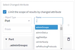
Note: For more details on the attributes (objects) and their properties, see the Cisco Crosswork Hierarchical Controller SHQL User Guide.
8. Click Get Report.
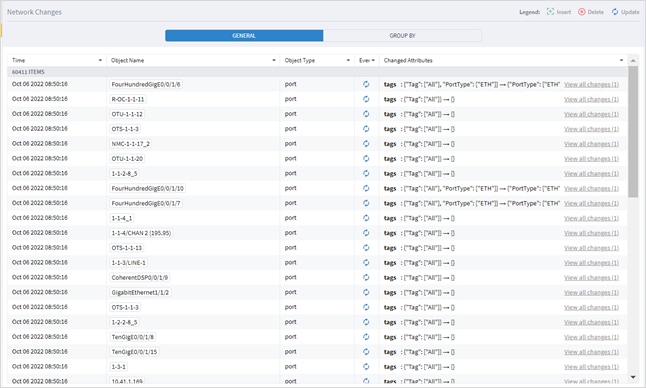
9. For an event, click in the Changed Attributes column to see the changes, for example,
tags : {} {"vendor": ["Ciena"]} means that a new tag was added to the resource with key=Vendor and value=Ciena.
![]()
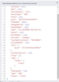
10. To view the full details of the resource as it is currently, click the row in table to get a JSON view of all attributes.
11. (Optional) To filter the results, click ![]() next to the field name, select the required values, and then click Apply.
next to the field name, select the required values, and then click Apply.
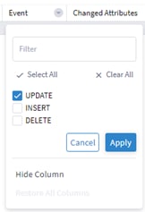
12. (Optional) To hide a column, click ![]() next to the field name, and then click Hide Column.
next to the field name, and then click Hide Column.
13. (Optional) To restore all columns, click ![]() next to any of the field names, and then click Restore All Columns.
next to any of the field names, and then click Restore All Columns.
Note: Hiding and restoring columns applies to all reports, not only to the open report..
14. (Optional) To view an object in the Explorer, click in the Object GUID column.
15. To save the report for future use, click ![]() Save.
Save.
![]()
16. Enter a report name and click Save.
You can use an existing report, edit the report, save the report with a new name, or delete the report.
To use an existing network history report:
1. In the applications bar, select Network History.
2. Click ![]() Open and select the required report.
Open and select the required report.
3. (Optional) Modify the report if required.
4. Click Get Report.
5. (Optional) If you want to save the report with a new name, click ![]() Save As.
Save As.
6. (Optional) If you want to delete a report, click ![]() Delete. A confirmation appears. Click Delete Report.
Delete. A confirmation appears. Click Delete Report.
Once you have run the history query, you can group the history report by time, object type or event.
To group the network history report:
1. In the applications bar, select Network History.
2. Fill in the Query Form and click Get Report.
3. Select the Group By tab.
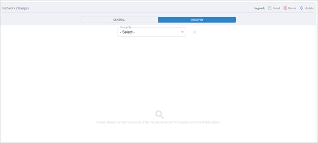
4. Select how to group the report:
◦ By Time: Select this option to count the number of events per second.
◦ By Object Type: Select this option to count the number of events per object type.
◦ By Event: Select this option to count the number of events of type insert, delete and update.
5. To view the detail for the group, select the required item. The details appear below.