FlashStack for Enterprise RAG Pipeline with NVIDIA NIM, NIM Operator, and RAG Blueprint
Available Languages
Bias-Free Language
The documentation set for this product strives to use bias-free language. For the purposes of this documentation set, bias-free is defined as language that does not imply discrimination based on age, disability, gender, racial identity, ethnic identity, sexual orientation, socioeconomic status, and intersectionality. Exceptions may be present in the documentation due to language that is hardcoded in the user interfaces of the product software, language used based on RFP documentation, or language that is used by a referenced third-party product. Learn more about how Cisco is using Inclusive Language.
- US/Canada 800-553-2447
- Worldwide Support Phone Numbers
- All Tools
 Feedback
 Feedback


About the Cisco Validated Design Program
The Cisco Validated Design (CVD) program consists of systems and solutions designed, tested, and documented to facilitate faster, more reliable, and more predictable customer deployments. For more information, go to: http://www.cisco.com/go/designzone.
Executive Summary
The Generative AI revolution necessitates secure integration with unique enterprise data to realize its full potential. Retrieval Augmented Generation (RAG) is the pivotal technology for this, yet deploying robust, enterprise-grade RAG pipelines has traditionally presented significant complexity, prolonged timelines, and considerable integration challenges.
This document introduces a Cisco Validated Design (CVD), specifically engineered to simplify, and accelerate the deployment of advanced RAG solutions. The design synergistically integrates the best-in-class FlashStack converged infrastructure—a high-performance foundation of Cisco UCS X-Series compute, Nexus networking, and Pure Storage FlashArray and FlashBlade—with NVIDIA's cutting-edge AI platform. This platform features the NVIDIA RAG Blueprint, providing a foundational structure with extensive customization freedom for tailoring pipelines to specific enterprise needs, and utilizes NVIDIA Inference Microservices (NIM) ensuring maximally optimized execution of AI inference tasks on the underlying NVIDIA GPUs. Orchestrated on Red Hat OpenShift Container Platform and managed via Cisco Intersight, this integrated system constitutes a dedicated AI enablement platform.
Lengthy integration cycles and associated deployment uncertainties are substantially mitigated by this approach. The validated blueprint provides a fast track for deploying powerful, private RAG pipelines, constructed upon meticulously tested, enterprise-grade components. This solution empowers enterprises to unlock their data's potential, establish trustworthy AI applications, and achieve a competitive advantage with unprecedented speed and operational confidence. This guide provides the detailed RAG design, while the FlashStack with Red Hat OpenShift Container and Virtualization Platform using Cisco UCS X-Series CVD offers the core infrastructure specifications.
If you are interested in understanding the FlashStack design and deployment details, including configuration of various elements of design and associated best practices, refer to the Cisco Validated Designs for FlashStack here: https://www.cisco.com/c/en/us/solutions/design-zone/data-center-design-guides/data-center-design-guides-all.html#FlashStack.
Solution Overview
This chapter contains the following:
● Audience
As enterprises seek to harness Generative AI with their proprietary data, Retrieval Augmented Generation (RAG) emerges as a critical technique. RAG enhances Large Language Models (LLMs) by grounding them in specific enterprise information, enabling accurate, context-aware responses for use cases like internal knowledge base querying. However, deploying robust, scalable, and secure RAG pipelines presents significant infrastructure and integration challenges.
This document introduces a Cisco validated solution addressing these challenges: Enterprise RAG Pipeline on FlashStack, leveraging NVIDIA RAG Blueprint and NVIDIA NIMs. This collaborative solution, jointly engineered by Cisco, Pure Storage and NVIDIA, provides a pre-integrated and optimized stack for deploying demanding GenAI workloads.
The foundation is FlashStack converged infrastructure. Layered upon this infrastructure is the NVIDIA AI software stack. The solution utilizes the NVIDIA RAG Blueprint, a reference architecture that accelerates the development of customizable RAG pipelines. This blueprint leverages NVIDIA Inference Microservices (NIM) – optimized, self-hosted endpoints for LLM inferencing, text embedding, and reranking – ensuring data privacy and low latency. NIMs are deployed and managed using the NIM Operator on Red Hat OpenShift Container Platform, orchestrated across NVIDIA GPU-accelerated Cisco UCS servers.
By integrating these best-in-class components into a Cisco Validated Design (CVD), this solution offers enterprises a streamlined path to deploying powerful, private RAG capabilities, reducing operational complexity, and accelerating time-to-value for GenAI initiatives.
The intended audience of this document includes IT decision makers such as CTOs and CIOs, IT architects, sales engineers, field consultants, professional services, IT managers, partner engineers, and customers. It is designed for those interested in the design, deployment, and life cycle management of Retrieval Augmented Generation pipelines with Cisco AI ready datacenter.
This document provides design and deployment guidance set up Retrieval Augmented Generation pipeline that uses NVIDIA NIM and GPU-accelerated components on FlashStack Datacenter.
The following design elements are built on the CVD FlashStack with Red Hat OCP Bare Metal Manual Configuration with Cisco UCS X-Series Direct Deployment Guide to implement an end-to-end Retrieval Augmented Generation pipeline using NVIDIA RAG Blueprint and NVIDIA NIMs.
● Installation and configuration of RAG pipeline components on FlashStack:
◦ NVIDIA GPUs
◦ NVIDIA AI Enterprise (NVAIE)
◦ NVIDIA NIM Operator
◦ NVIDIA NIM microservices - NVIDIA NIMs for LLM Inferencing, text embedding and text reranking.
◦ NVIDIA AI Blueprint version 1.0.0 for RAG
◦ RAG Evaluation
◦ NIM for LLM Benchmarking
◦ Vector Database Benchmarking
This solution provides a validated, foundational architecture for deploying enterprise-grade Retrieval Augmented Generation pipelines. It leverages a Cisco UCS X-Series based FlashStack Datacenter as the high-performance converged infrastructure foundation. Key NVIDIA AI technologies, including the RAG Blueprint reference implementation and NVIDIA Inference Microservices (NIM) running on NVIDIA GPUs, power the AI workload. NVIDIA NIM Operator manages the life cycle of the NVIDIA NIM for LLMs, Text Embedding NIM and Reranking NIMs.
The entire stack is deployed on a bare-metal Red Hat OpenShift cluster, utilizing Portworx by Pure Storage for container-native persistent storage. This pre-tested integration of validated models, GPUs, and backend components, accessible via NIM's industry-standard APIs, delivers an optimized and AI-ready platform, significantly simplifying the deployment and management of secure, private RAG applications.
This architecture represents a rigorously tested and validated integration across all layers – compute, networking, storage, NVIDIA GPUs, AI models, and the software stack (OCP, Portworx, NVIDIA AI Enterprise). NVIDIA NIM facilitates streamlined application development and integration via industry-standard APIs (including OpenAI compatibility). The resultant platform is an optimized, secure, and AI-ready infrastructure solution designed to mitigate deployment complexities, reduce operational overhead, and accelerate the delivery of high-performance, private RAG capabilities within the enterprise.
Figure 1 illustrates the solution overview.
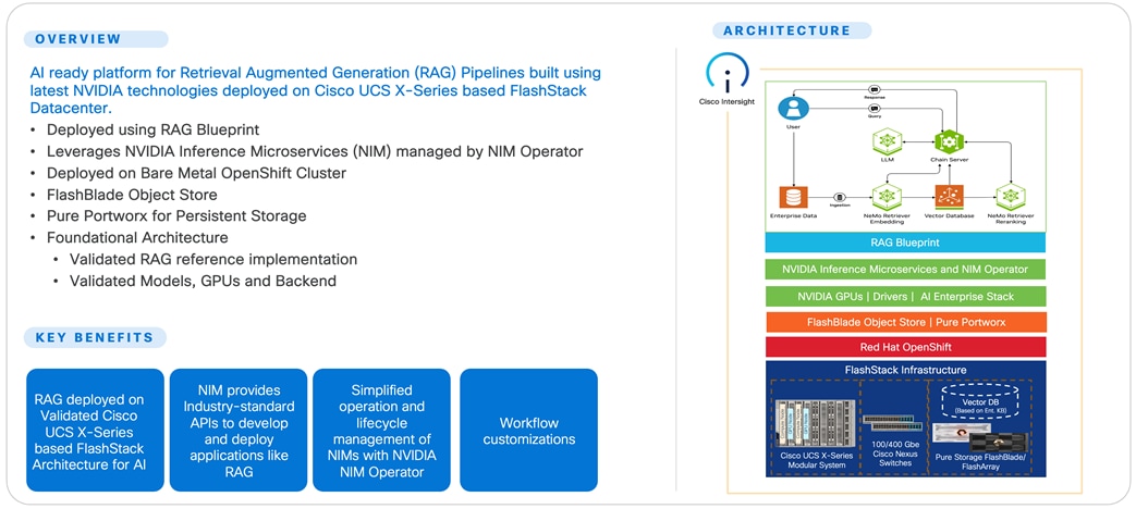
The FlashStack solution as a platform for Retrieval Augmented Generation offers the following key benefits:
● The ability to implement a Retrieval Augmented Generation pipeline quickly and easily on a powerful platform with high-speed persistent storage.
● Blueprint leverages NVIDIA NIM microservices deployed on-premise to meet specific data governance and latency requirements.
● Evaluation of performance of platform components.
● Simplified cloud-based management of solution components using policy-driven modular design.
● Cooperative support model and Cisco Solution Support.
● Easy to deploy, consume, and manage architecture, which saves time and resources required to research, procure, and integrate off-the-shelf components.
● Support for component monitoring, solution automation and orchestration, and workload optimization.
Like all other FlashStack solution designs, FlashStack for Enterprise RAG Pipeline with NVIDIA NIM, NIM Operator and RAG Blueprint is configurable according to demand and usage. You can purchase exactly the infrastructure you need for your current application requirements and then scale-up/scale-out to meet future needs.
Technology Overview
This chapter contains the following:
● Retrieval Augmented Generation
● NVIDIA Inference Microservices
● NVIDIA NIM for Large Language Models
● Benefits of Portworx Enterprise with OpenShift Container Platform
● Benefits of Portworx Enterprise with Pure Storage FlashArray
● Benefits of Pure Storage FlashBlade
Retrieval Augmented Generation
Retrieval Augmented Generation (RAG) is an enterprise application of Generative AI. RAG represents a category of large language model (LLM) applications that enhance the LLM's context by incorporating external data. It overcomes the limitation of knowledge cutoff date (events occurring after the model’s training). LLMs lack access to an organization's internal data or services. This absence of up-to-date and domain-specific or organization-specific information prevents their effective use in enterprise applications.
RAG Pipeline
Figure 2 illustrates the RAG Pipeline overview.
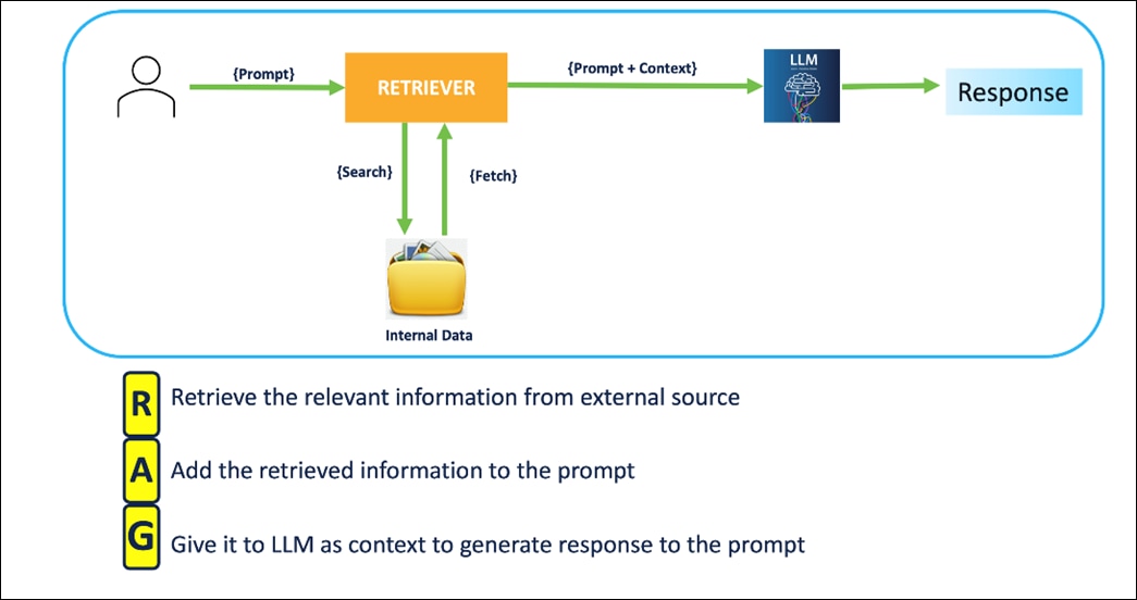
In this pipeline, when you enter a prompt/query, document chunks relevant to the prompt are searched and fetched to the system. The retrieved relevant information is augmented to the prompt as context. LLM is asked to generate a response to the prompt in the context and the user receives the response.
RAG Architecture
RAG is an end-to-end architecture that combines information retrieval component with a response generator.
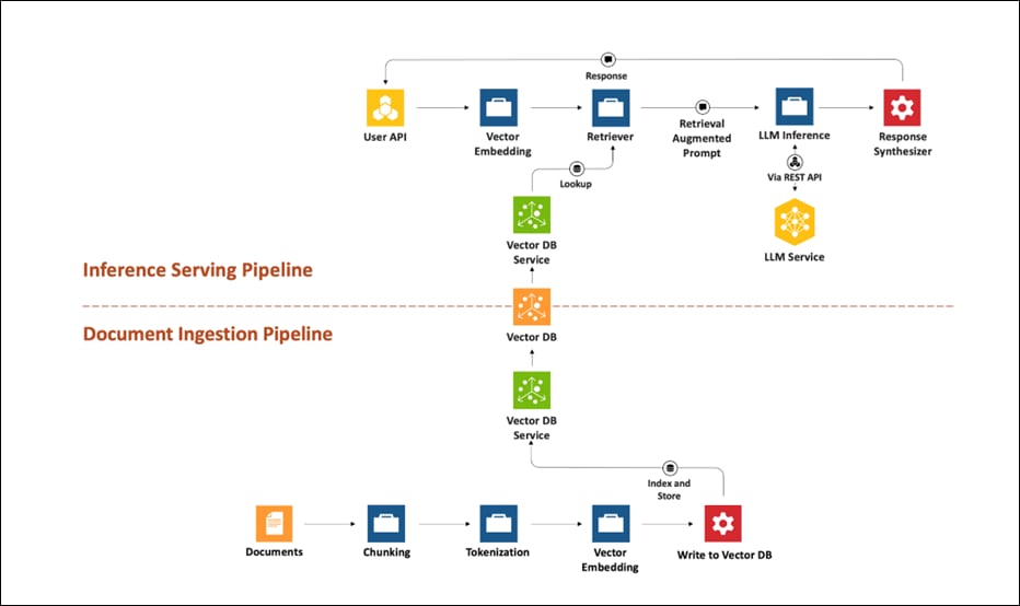
RAG can be broken into two process flows; document ingestion and inferencing.
Figure 4 illustrates the document ingestion pipeline.
Figure 5 illustrates the inferencing pipeline.
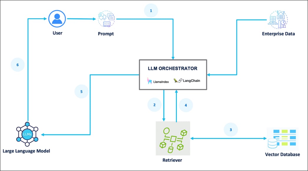
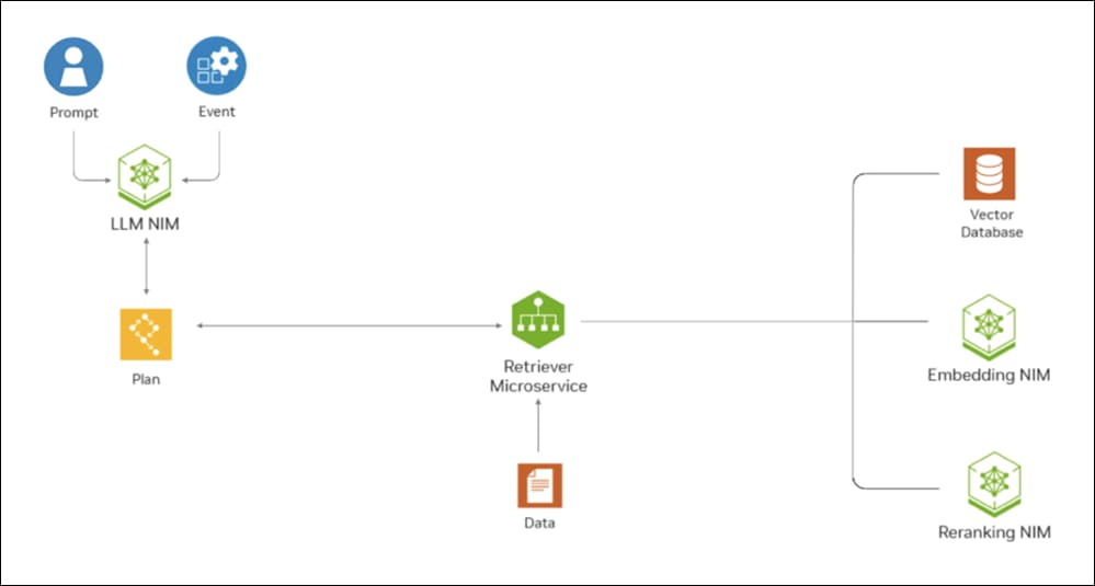
The process for the inference serving pipeline is as follows:
1. A prompt is passed to the LLM orchestrator.
2. The orchestrator sends a search query to the retriever.
3. The retriever fetches relevant information from the Vector Database.
4. The retriever returns the retrieved information to the orchestrator.
5. The orchestrator augments the original prompt with the context and sends it to the LLM.
6. The LLM responds with generated text/ response and presents it to the user.
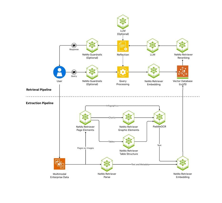
The NVIDIA AI Blueprint for RAG gives developers a foundational starting point for building scalable, customizable retrieval pipelines that deliver both high accuracy and throughput. Use this blueprint to build RAG applications that provide context-aware responses by connecting LLMs to extensive multimodal enterprise data—including text, tables, charts, and infographics from millions of PDFs. With 15x faster multimodal PDF data extraction and 50 percent fewer incorrect answers, enterprises can unlock actionable insights from data and drive productivity at scale.
This blueprint can be used as-is, combined with other NVIDIA Blueprints, such as the Digital Human blueprint or the AI Assistant for customer service blueprint, or integrated with an agent to support more advanced use cases. Get started with this reference architecture to ground AI-driven decisions in relevant enterprise data - wherever it resides.
The NVIDIA AI Enterprise (NVAIE) platform was deployed on Red Hat OpenShift as the foundation for the RAG pipeline. NVIDIA AI Enterprise simplifies the development and deployment of generative AI workloads, including Retrieval Augmented Generation, at scale.
NVIDIA Inference Microservices
NVIDIA Inference Microservice (NIM), a component of NVIDIA AI Enterprise, offers an efficient route for creating AI-driven enterprise applications and deploying AI models in production environments. NIM consists of microservices that accelerate and simplify the deployment of generative AI models via automation using prebuilt containers, Helm charts, optimized models, and industry-standard APIs.
NIM simplifies the process for IT and DevOps teams to self-host large language models (LLMs) within their own managed environments. It provides developers with industry-standard APIs, enabling them to create applications such as copilots, chatbots, and AI assistants that can revolutionize their business operations. Content Generation, Sentiment Analysis, and Language Translation services are just a few additional examples of applications that can be rapidly deployed to meet various use cases. NIM ensures the quickest path to inference with unmatched performance.
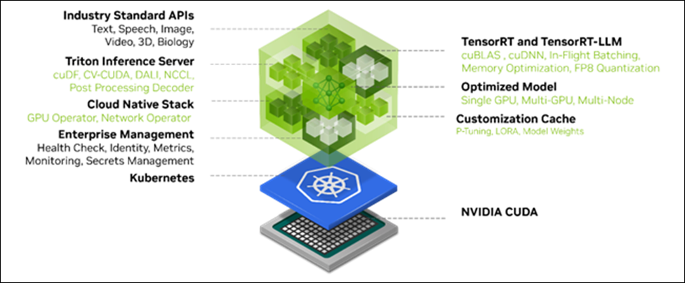
NIMs are distributed as container images tailored to specific models or model families. Each NIM is encapsulated in its own container and includes an optimized model. These containers come with a runtime compatible with any NVIDIA GPU that has adequate GPU memory, with certain model/GPU combinations being optimized for better performance. One or more GPUs can be passed through to containers via the NVIDIA Container Toolkit to provide the horsepower needed for any workload. NIM automatically retrieves the model from NGC (NVIDIA GPU Cloud), utilizing a local filesystem cache if available. Since all NIMs are constructed from a common base, once a NIM has been downloaded, acquiring additional NIMs becomes significantly faster. The NIM catalog currently offers nearly 150 models and agent blueprints.
Utilizing domain specific models, NIM caters to the demand for specialized solutions and enhanced performance through a range of pivotal features. It incorporates NVIDIA CUDA (Compute Unified Device Architecture) libraries and customized code designed for distinct fields like language, speech, video processing, healthcare, retail, and others. This method ensures that applications are precise and pertinent to their particular use cases. Think of it like a custom toolkit for each profession; just as a carpenter has specialized tools for woodworking, NIM provides tailored resources to meet the unique needs of various domains.
NIM is designed with a production-ready base container that offers a robust foundation for enterprise AI applications. It includes feature branches, thorough validation processes, enterprise support with service-level agreements (SLAs), and frequent security vulnerability updates. This optimized framework makes NIM an essential tool for deploying efficient, scalable, and tailored AI applications in production environments. Think of NIM as the bedrock of a skyscraper; just as a solid foundation is crucial for supporting the entire structure, NIM provides the necessary stability and resources for building scalable and reliable portable enterprise AI solutions.
NVIDIA NIM for Large Language Models
NVIDIA NIM for Large Language Models (LLMs) (NVIDIA NIM for LLMs) brings the power of state-of-the-art large language models (LLMs) to enterprise applications, providing unmatched natural language processing (NLP) and understanding capabilities.
Whether developing chatbots, content analyzers, or any application that needs to understand and generate human language — NVIDIA NIM for LLMs is the fastest path to inference. Built on the NVIDIA software platform, NVIDIA NIM brings state of the art GPU accelerated large language model serving.
High Performance Features
NVIDIA NIM for LLMs abstracts away model inference internals such as execution engine and runtime operations. NVIDIA NIM for LLMs provides the most performant option available whether it be with TensorRT, vLLM or LLM others.
● Scalable Deployment: NVIDIA NIM for LLMs is performant and can easily and seamlessly scale from a few users to millions.
● Advanced Language Models: Built on cutting-edge LLM architectures, NVIDIA NIM for LLMs provides optimized and pre-generated engines for a variety of popular models. NVIDIA NIM for LLMs includes tooling to help create GPU optimized models.
● Flexible Integration: Easily incorporate the microservice into existing workflows and applications. NVIDIA NIM for LLMs provides an OpenAI API compatible programming model and custom NVIDIA extensions for additional functionality.
● Enterprise-Grade Security: Data privacy is paramount. NVIDIA NIM for LLMs emphasizes security by using safetensors, constantly monitoring and patching CVEs in our stack and conducting internal penetration tests.
Applications
The potential applications of NVIDIA NIM for LLMs are vast, spanning across various industries and use cases:
● Chatbots & Virtual Assistants: Empower bots with human-like language understanding and responsiveness.
● Content Generation & Summarization: Generate high-quality content or distill lengthy articles into concise summaries with ease.
● Sentiment Analysis: Understand user sentiments in real-time, driving better business decisions.
● Language Translation: Break language barriers with efficient and accurate translation services.
Architecture
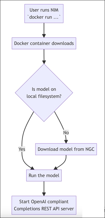
NVIDIA NIM for LLMs is one of what will become many NIMs. Each NIM has its own Docker container with a model, such as meta/llama3-8b-instruct. These containers include the runtime capable of running the model on any NVIDIA GPU. The NIM automatically downloads the model from NGC, leveraging a local filesystem cache if available. Each NIM is built from a common base, so once a NIM has been downloaded, downloading additional NIMs is extremely fast.
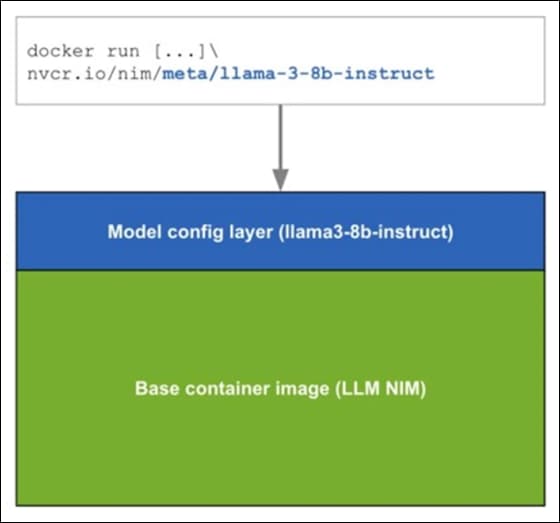
When a NIM is first deployed, NIM inspects the local hardware configuration, and the available optimized model in the model registry, and then automatically chooses the best version of the model for the available hardware. For a subset of NVIDIA GPUs, see: Support Matrix, NIM downloads the optimized TRT (TensorRT) engine and runs an inference using the TRT-LLM library. For all other NVIDIA GPUs, NIM downloads a non-optimized model and runs it using the vLLM library.
NIMs are distributed as NGC container images through the NVIDIA NGC Catalog. A security scan report is available for each container within the NGC catalog, which provides a security rating of that image, breakdown of CVE severity by package, and links to detailed information on CVEs.
Deployment Lifecycle
Figure 9 illustrates the deployment lifecycle.
NeMo Text Retriever NIM APIs facilitate access to optimized embedding models — essential components for RAG applications that deliver precise and faithful answers. By using NVIDIA software (including CUDA, TensorRT, and Triton Inference Server), the Text Retriever NIM provides the tools needed by developers to create ready-to-use, GPU-accelerated applications. NeMo Retriever Text Embedding NIM enhances the performance of text-based question-answering retrieval by generating optimized embeddings. For this RAG CVD, the Snowflake Arctic-Embed-L embedding model was harnessed to encode domain-specific content which was then stored in a vector database. The NIM combines that data with an embedded version of the user’s query to deliver a relevant response.
Figure 10 shows how the Text Retriever NIM APIs can help a question-answering RAG application find the most relevant data in an enterprise setting.
Enterprise-Ready Features
Text Embedding NIM comes with enterprise-ready features, such as a high-performance inference server, flexible integration, and enterprise-grade security.
● High Performance: Text Embedding NIM is optimized for high-performance deep learning inference with NVIDIA TensorRT and NVIDIA Triton Inference Server.
● Scalable Deployment: Text Embedding NIM seamlessly scales from a few users to millions.
● Flexible Integration: Text Embedding NIM can be easily incorporated into existing data pipelines and applications. Developers are provided with an OpenAI-compatible API in addition to custom NVIDIA extensions.
● Enterprise-Grade Security: Text Embedding NIM comes with security features such as the use of safetensors, continuous patching of CVEs, and constant monitoring with our internal penetration tests.
The FlashStack architecture was jointly developed by Cisco and Pure Storage. All FlashStack components are integrated, allowing customers to deploy the solution quickly and economically while eliminating many of the risks associated with researching, designing, building, and deploying similar solutions from the foundation. One of the main benefits of FlashStack is its ability to maintain consistency at scale. Figure 11 illustrates the series of hardware components used for building the FlashStack architectures.
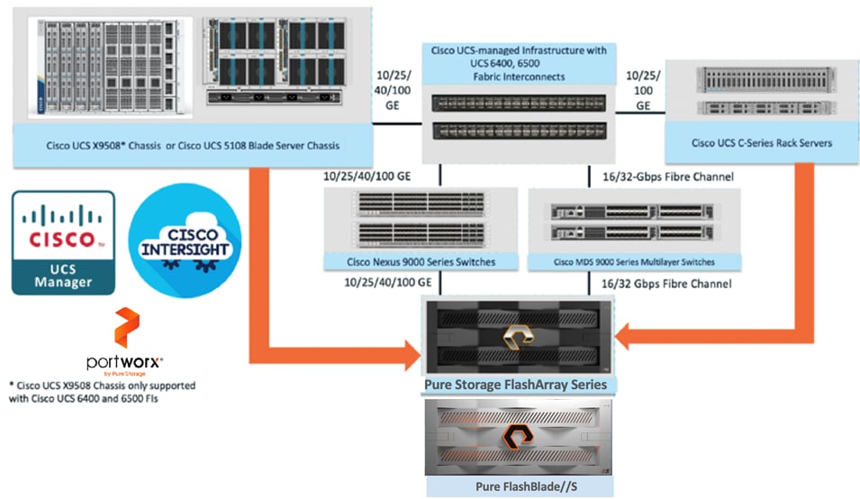
All FlashStack components are integrated, so you can deploy the solution quickly and economically while eliminating many of the risks associated with researching, designing, building, and deploying similar solutions from the foundation. One of the main benefits of FlashStack is its ability to maintain consistency at scale. Each of the component families shown in Figure 11 (Cisco UCS, Cisco Nexus, Cisco MDS, Portworx by Pure Storage, Pure Storage FlashArray and FlashBlade systems) offers platform and resource options to scale up or scale out the infrastructure while supporting the same features and functions.
Benefits of Portworx Enterprise with OpenShift Container Platform
Portworx Enterprise is a multi-cloud solution, providing cloud-native storage for workloads running anywhere, from on-prem to cloud to hybrid/multi-cloud environments. Portworx Enterprise is deployed on Red Hat OpenShift cluster using the Red Hat certified Portworx Enterprise operator, available on Red Hat’s OperatorHub. Portworx with Red Hat OpenShift Container Platform enhances data management for container workloads by offering integrated, enterprise-grade storage. It includes simplified storage operations through Kubernetes, high availability and resiliency across environments, advanced disaster recovery options, and automated scaling capabilities. This integration supports a unified infrastructure where traditional and modern workloads coexist, providing flexibility in deployment across diverse infrastructures and ensuring robust data security.
Portworx and Stork offer a combined solution for managing persistent data and stateful applications within Red Hat OpenShift (OCP), providing features like storage orchestration, disaster recovery, and data protection. Portworx provides a software-defined storage solution that works natively within Kubernetes, including OpenShift, while Stork acts as a storage scheduler and orchestrator, enhancing the functionality of Portworx.
Benefits of Portworx Enterprise with Pure Storage FlashArray
Portworx on FlashArray offers flexible storage deployment options for Kubernetes. Using FlashArray as cloud drives enables automatic volume provisioning, cluster expansion, and supports PX Backup and Autopilot. Direct Access volumes allow for efficient on-premises storage management, offering file system operations, IOPS, and snapshot capabilities. Multi-tenancy features isolate storage access per user, enhancing security in shared environments.
Portworx on FlashArray enhances Kubernetes environments with robust data reduction, resiliency, simplicity, and support. It lowers storage costs through deduplication, compression, and thin provisioning, providing 2-10x data reduction. FlashArray’s reliable infrastructure ensures high availability, reducing server-side rebuilds. Portworx simplifies Kubernetes deployment with minimal configuration and end-to-end visibility via Pure1. Additionally, unified support, powered by Pure1 telemetry, offers centralized, proactive assistance for both storage hardware and Kubernetes services, creating an efficient and scalable solution for enterprise needs.
Benefits of Pure Storage FlashBlade
Pure Storage FlashBlade//S is a scale-out storage system that is designed to grow with your unstructured data needs for AI/ML, analytics, high performance computing (HPC), and other data-driven file and object use cases in areas of healthcare, genomics, financial services, and more. FlashBlade//S provides a simple, high-performance solution for Unified Fast File and Object (UFFO) storage with an all-QLC based, distributed architecture that can support NFS, SMB, and S3 protocol access. The cloud-based Pure1® data management platform provides a single view to monitor, analyze, and optimize storage from a centralized location.
FlashBlade//S is the ideal data storage platform for AI, as it was purpose-built from the ground up for modern, unstructured workloads and accelerates AI processes with the most efficient storage platform at every step of your data pipeline. A centralized data platform in a deep learning architecture increases the productivity of AI engineers and data scientists and makes scaling and operations simpler and more agile for the data architect.
An AI project that uses a single-chassis system during early model development can expand non-disruptively as data requirements grow during training and continue to expand as more live data is accumulated during production.
Table 1. FlashBlade//S Specifications
| FlashBlade |
Scalability |
Capacity |
Connectivity |
Physical |
| FlashBlade//S |
Start with a minimum of 7 blades and scale up to 10 blades in a single chassis |
Up to 4 DirectFlash Modules per blade (24TB or 37TB or 48TB or 75TB DirectFlash Modules) |
Uplink networking 8 x 100GbE |
5U per chassis Dimensions: 8.59” x 17.43” x 32.00” x 32.00” |
| Independently scale capacity and performance with all-QLC architecture |
Up to 300TB per blade |
Future-proof midplane |
2,400W (nominal at full configuration) |
Solution Design
This chapter contains the following:
● Red Hat OpenShift Container Platform on Bare Metal Server Configuration
The FlashStack Datacenter with Cisco UCS and Cisco Intersight meets the following general design requirements:
● Resilient design across all the layers of infrastructure with no single point of failure
● Scalable design with the flexibility to add compute capacity, storage, or network bandwidth as needed
● Modular design that can be replicated to expand and grow as the needs of the business grow
● Flexible design that can support different models of various components with ease
● Simplified design with the ability to integrate and automate with external automation tools
● Cloud-enabled design which can be configured, managed, and orchestrated from the cloud using GUI or APIs
● Repeatable design for accelerating the provisioning of end-to-end Retrieval Augmented Generation pipeline
● Provide a testing methodology to evaluate the performance of the solution
● Provide an example implementation of Cisco Webex Chat Bot integration with RAG
To deliver a solution which meets all these design requirements, various solution components are connected and configured as explained in the following sections.
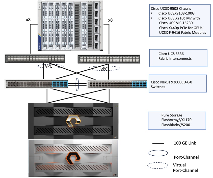
The FlashStack for Accelerated RAG Pipeline with NVIDIA NIM and NIVIDIA Blueprint is built using the following reference hardware components:
● One Cisco UCS X9508 chassis, equipped with a pair of Cisco UCS X9108 100G IFMs, contains six Cisco UCS X210c M7 compute nodes and two Cisco UCS X440p PCIe nodes each with two NVIDIA L40S GPUs. Other configurations of servers with and without GPUs are also supported. Each compute node is equipped with fifth-generation Cisco VIC card 15231 providing 100-G ethernet connectivity on each side of the fabric. A pair of Fabric Modules installed at the rear side of the chassis enables connectivity between the X440p PCIe nodes and X210c M7 nodes.
● Cisco fifth-generation 6536 fabric interconnects are used to provide connectivity to the compute nodes installed in the chassis.
● High-speed Cisco NXOS-based Nexus C93600CD-GX switching design to support up to 100 and 400-GE connectivity.
● FlashBlade//S200 is used as S3 compatible object storage to persist Milvus Vector database large-scale files, such as index files and binary logs. It is directly exposed to Milvus vector database pods hosted on the OpenShift cluster. The OpenShift cluster is configured to route the object storage traffic from Milvus Pods to FlashBlade via worker node’s object storage network interface. Pure Storage FlashBlade is a unified and scale out storage platform providing native file and object storage, offering a modular architecture for unstructured data workloads, enabling independent scaling of compute and capacity.
● FlashArray//XL170 is used as high performing back end storage for Portworx Enterprise which provides cloud native persistent storage with enterprise grade features for containers and other workloads running on the OpenShift cluster.
Figure 12 shows the physical topology and network connections used for this Ethernet-based FlashStack design.
The software components consist of:
● Cisco Intersight platform to deploy, maintain, and support the FlashStack components.
● Cisco Intersight Assist virtual appliance to help connect the Pure Storage FlashArray and Cisco Nexus Switches with the Cisco Intersight platform to enable visibility into these platforms from Intersight.
● Red Hat OpenShift Container Platform for providing a consistent hybrid cloud foundation for building and scaling containerized and virtualized applications.
● Portworx by Pure Storage (Portworx Enterprise) data platform for providing enterprise grade storage for containerized workloads hosted on OpenShift platform.
● Pure Storage Pure1 is a cloud-based, AI-driven SaaS platform that simplifies and optimizes data storage management for Pure Storage arrays, offering features like proactive monitoring, predictive analytics, and automated tasks.
The information in this section is provided as a reference for cabling the physical equipment in a FlashStack environment.
Compute Infrastructure Design
The compute infrastructure in FlashStack solution consists of the following:
● Cisco UCS X210c M7 Compute Nodes
● Cisco UCS X-Series chassis (Cisco UCSX-9508) with Intelligent Fabric Modules (Cisco UCSX-I-9108-25G)
● Cisco UCS Fabric Interconnects (Cisco UCS-FI-6536)
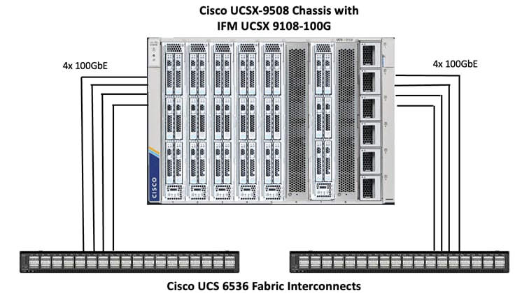
Compute System Connectivity
The Cisco UCS X9508 Chassis is equipped with the Cisco UCSX 9108-100G intelligent fabric modules (IFMs). The Cisco UCS X9508 Chassis connects to each Cisco UCS 6536 FI using four 100GE ports, as shown in Figure 13. If you require more bandwidth, all eight ports on the IFMs can be connected to each FI.
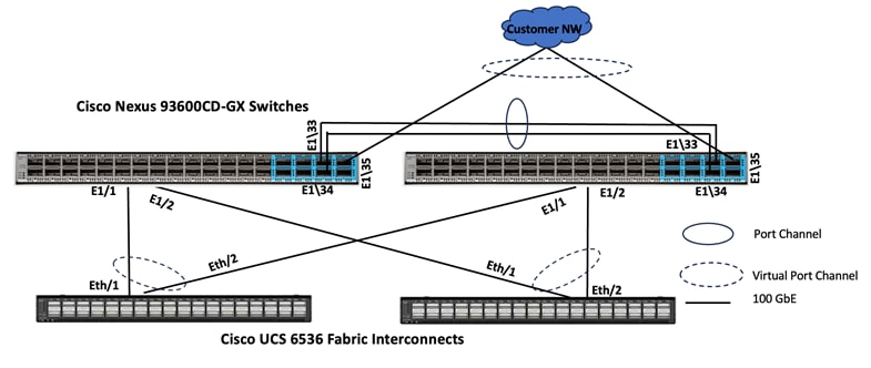
Compute UCS Fabric Interconnect 6536 Ethernet Connectivity
Cisco UCS 6536 FIs are connected to Cisco Nexus 93600CD-GX switches using 100GE connections configured as virtual port channels. Each FI is connected to both Cisco Nexus switches using a 100G connections; additional links can easily be added to the port channel to increase the bandwidth as needed. Below figure illustrates the physical connectivity details.
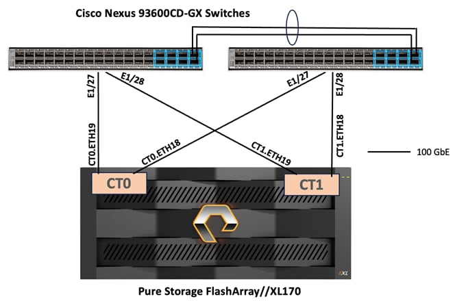
Pure Storage FlashArray//XL170 Ethernet Connectivity
Pure Storage FlashArray controllers are connected to Cisco Nexus 93600CD-GX switches using redundant 100-GE. Figure 15 illustrates the physical connectivity details.
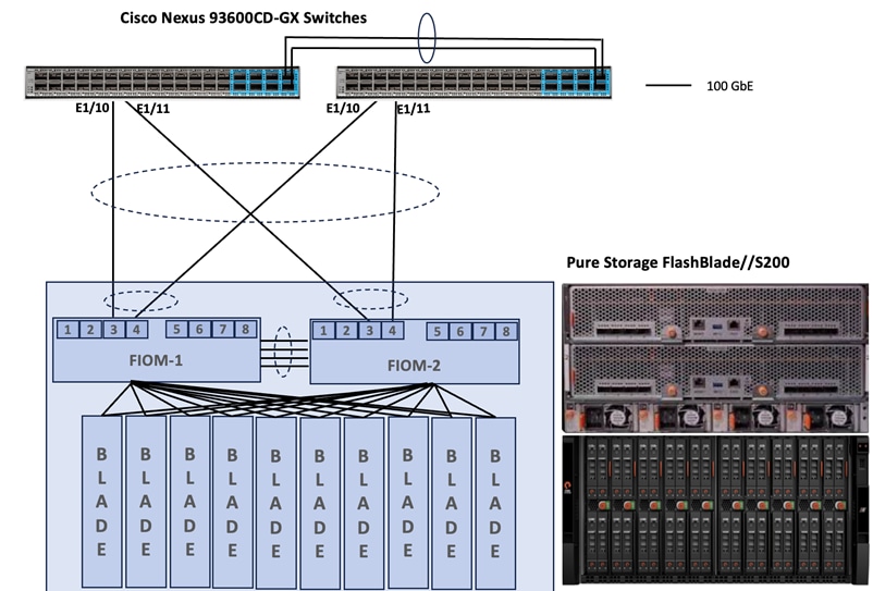
Pure Storage FlashBlade//S200 Ethernet Connectivity
Pure Storage FlashBlade uplink ports (2x 100GbE from each FIOM) are connected to Cisco Nexus 93600CD-GX switches as shown in Figure 16. Additional links can easily be added (up to 8x 100GbE on each FIOM) to the port channel to increase the bandwidth as needed. Following figure illustrates the physical connectivity details.
Note: Additional 1Gb management connections are needed for one or more out-of-band network switches that are apart from the FlashStack infrastructure. Each Cisco UCS fabric interconnect and Cisco Nexus switch is connected to the out-of-band network switches, Pure Storage FlashArray controllers and FlashBlade//S200 have connections to the out-of-band network switches. Layer 3 network connectivity is required between the Out-of-Band (OOB) and In-Band (IB) Management Subnets.
Red Hat OpenShift Container Platform on Bare Metal Server Configuration
A simple Red Hat OpenShift cluster consists of at least five servers – 3 Master or Control Plane Nodes and 2 or more Worker or compute Nodes where applications and VMs are run. In this lab validation 3 Worker Nodes were utilized. Based on published Red Hat requirements, the three Master Nodes were configured with 64GB RAM, and the three Worker Nodes were configured with 1024GB memory to handle containerized applications and Virtual Machines. Each Node was booted from RAID1 disk created using two M.2 SSD drives. Also, the servers paired with X440p PCIe Nodes were configured as Workers. From a networking perspective, both the Masters and the Workers were configured with a single vNIC with UCS Fabric Failover in the Bare Metal or Management VLAN. The Workers were configured with extra NICs (vNICs) to allow storage attachment to the Workers.
Each worker node is configured with two additional vNICs with the iSCSI A and B VLANs tagged as native to allow iSCSI persistent storage attachment from FlashArray//XL170 and future iSCSI boot. Finally, each worker is also configured with one additional vNIC with the OCP Object-Storage VLAN tagged as native VLAN to provide object persistent storage from FlashBlade//S200.
Worker Node Network Configuration
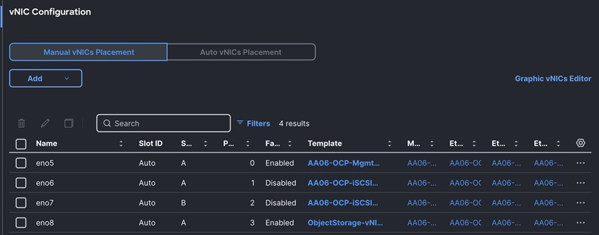
The worker node is configured with four vNICs. The first three vNICs are used by worker node for OpenShift cluster management traffic (eno5) and storage traffic using iSCSI protocol (eno6 and eno7). While the last vNIC (eno8) is used for object storage traffic over ethernet. vNICs eno5 and eno8 vNICs are configured with Fabric-Failover option while the vNICs eno6 and eno7 are used as independent interfaces for iSCSI storage traffic via Fabric-A and B, respectively. The following figure illustrates the vNIC configuration of OpenShift worker nodes.
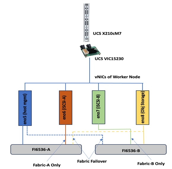
The control plane (master node) will just have one vNIC eno5 with Fabric-Failover option enabled. This vNIC is used to carry the worker management and OCP cluster traffic.
VLAN Configuration
Table 2 lists the VLANs configured for setting up the FlashStack environment along with their usage.
| VLAN ID |
NAME |
Usage |
IP Subnet used in this deployment |
| 2 |
Native-VLAN |
VLAN2 is used as native VLAN instead of default VLAN1 |
|
| 1060 |
OOB-Mgmt-VLAN |
Out-of-band management VLAN to connect management port for various devices |
10.106.0.24/0 BW: 10.106.0.254 |
| 1061 |
IB-Mgmt-VLAN |
Routable Bare Metal VLAN used for OpenShift cluster and node management |
10.106.1.0/24 GW: 10.106.1.254 |
| 3010 |
OCP-iSCSI-A |
Used for OpenShift iSCSI persistent storage via Fabric-A |
192.168.51.0/24 |
| 3020 |
OCP-iSCSI-B |
Used for OpenShift iSCSI persistent storage via Fabric-B |
192.168.52.0/24 |
| 3040 |
OCP-Object-storage |
Used for Object Storage traffic |
192.168.40.0/24 |
Table 3 lists the infrastructure services running on either virtual machines or bar mental servers required for deployment as outlined in the document. All these services are hosted on pre-existing infrastructure with in the FlashStack
Table 3. Infrastructure services
| Service Description |
VLAN |
IP Address |
| AD/DNS-1 & DHCP |
1061 |
10.106.1.21 |
| AD/DNS-2 |
1061 |
10.106.1.22 |
| OCP installer/bastion node |
1061 |
10.106.1.23 |
| Cisco Intersight Assist Virtual Appliance |
1061 |
10.106.1.24 |
Software Revisions
The FlashStack Solution with Red Hat OpenShift on Bare Metal infrastructure configuration is built using the following components.
Table 4 lists the required software revisions for various components of the solution.
| Layer |
Device |
Image Bundle version |
Comments |
| Compute |
Pair of Cisco UCS Fabric Interconnect – 6530 |
4.3(4.240066) |
|
|
|
6x Cisco UCS X210 M7 with Cisco VIC 15230 |
5.2(2.240053) |
|
| Network |
Cisco Nexus 93699CD-GX-NX-OS |
10.3(5)(M) |
|
| Storage |
Pure Storage FlashArray Purity //FA Pure Storage FlashBlade//S200 |
Purity//FA 6.6.10 Purity//FB 4.1.12 |
|
| Software |
Red Hat OpenShift |
4.17 |
|
|
|
Portworx Enterprise |
3.1.6 |
|
|
|
Cisco Intersight Assist Appliance |
1.1.1-0 |
|
|
|
NVIDIA L40S Driver |
550.90.07 |
|
This solution implements a validated Retrieval Augmented Generation (RAG) pipeline architected to enhance Large Language Model (LLM) capabilities with real-time access to enterprise-specific data, thereby increasing user trust and mitigating hallucinations. The design adheres to core RAG principles aligning with the robust methodologies.
This entire RAG pipeline is deployed upon a validated FlashStack architecture, specifically configured following the best practices outlined here: FlashStack with Red Hat OpenShift Container and Virtualization Platform using Cisco UCS X-Series Design and Deployment Guide.
The layered infrastructure, running on Red Hat OpenShift Container Platform with persistent storage managed by Portworx Enterprise, provides a high-performance, secure, and scalable environment. The use of locally deployed NVIDIA NIMs within this secure infrastructure ensures data privacy and control.
This design leverages the NVIDIA RAG Blueprint as a foundational framework, implemented with optimized NVIDIA NIMs. It directly addresses the goals of RAG by providing up-to-date, proprietary information to the LLM securely. The underlying FlashStack platform offers significant performance and reliability, while also being extensible for future AI initiatives such as model fine-tuning, training, or other inferencing use cases, contingent on appropriate resource allocation.

Network Switch Configuration
This chapter contains the following:
● Cisco Nexus Switch Manual Configuration
● Claim Cisco Nexus Switches into Cisco Intersight
Physical cabling should be completed by following the diagram and table references in section FlashStack Cabling.
The following procedures describe how to configure the Cisco Nexus 93600CD-GX switches for use in a FlashStack environment. This procedure assumes the use of Cisco Nexus 9000 10.1(2), the Cisco suggested Nexus switch release at the time of this validation.
The procedure includes the setup of NTP distribution on both the mgmt0 port and the in-band management VLAN. The interface-vlan feature and ntp commands are used to set this up. This procedure also assumes that the default VRF is used to route the in-band management VLAN.
This document assumes that initial day-0 switch configuration is already done using switch console ports and ready to use the switches using their management IPs.
Cisco Nexus Switch Manual Configuration
Procedure 1. Enable features on Cisco Nexus A and Cisco Nexus B
Step 1. Log into both Nexus switches as admin using ssh.
Step 2. Enable the switch features as described below:
config t
feature nxapi
cfs eth distribute
feature udld
feature interface-vlan
feature netflow
feature hsrp
feature lacp
feature vpc
feature lldp
Procedure 2. Set Global Configurations on Cisco Nexus A and Cisco Nexus B
Step 1. Log into both Nexus switches as admin using ssh.
Step 2. Run the following commands to set the global configurations:
spanning-tree port type edge bpduguard default
spanning-tree port type edge bpdufilter default
spanning-tree port type network default
system default switchport
system default switchport shutdown
port-channel load-balance src-dst l4port
ntp server <Global-ntp-server-ip> use-vrf default
ntp master 3
clock timezone <timezone> <hour-offset> <minute-Offset>
clock summer-time <timezone> <start-weekk> <start-day> <start-month> <start-time> <end-week> <end-day> <enb-month> <end-time> <offset-minutes>
ip route 0.0.0.0/0 <IB-Mgmt-VLAN-gatewayIP>
copy run start
Note: It is important to configure the local time so that logging time alignment and any backup schedules are correct. For more information on configuring the timezone and daylight savings time or summer time, go to: https://www.cisco.com/c/en/us/td/docs/dcn/nx-os/nexus9000/102x/configuration/fundamentals/cisco-nexus-9000-nx-os-fundamentals-configuration-guide-102x/m-basic-device-management.html#task_1231769
Sample clock commands for the United States Eastern timezone are:
clock timezone EST -5 0
clock summer-time EDT 2 Sunday March 02:00 1 Sunday November 02:00 60
Procedure 3. Create VLANs on Cisco Nexus A and Cisco Nexus B
Step 1. From the global configuration mode, run the following commands:
Vlan <oob-mgmt-vlan-id>
name OOB-Mgmt-VLAN
Vlan <ib-mgmt-vlan-id>
name IB-Mgmt-VLAN
Vlan <native-vlan-id>
name Native-VLAN
Vlan <ocp-iscsi-a-vlan-id>
name OCP-iSCSI-A
Vlan <ocp-iscsi-b-vlan-id>
name OCP-iSCSI-B
Vlan <vm-mgmt-vlan-id>
name VM-Mgmt-VLAN
Procedure 4. Add NTP Distribution Interface
Cisco Nexus - A
Step 1. From the global configuration mode, run the following commands:
interface vlan <ib-mgmt-vlan-id>
ip address <switch-a-ntp-ip>/<ib-mgmt-vlan-netmask-length>
no shut
exit
ntp peer <switch-b-ntp-ip> use-vrf default
Cisco Nexus - B
Step 1. From the global configuration mode, run the following commands:
interface vlan <ib-mgmt-vlan-id>
ip address <switch-b-ntp-ip>/<ib-mgmt-vlan-netmask-length>
no shut
exit
ntp peer <switch-a-ntp-ip> use-vrf default
Procedure 5. Define Port Channels on Cisco Nexus A and Cisco Nexus B
Cisco Nexus – A and B
Step 1. From the global configuration mode, run the following commands:
interface port-channel 10
description vPC Peer Link
switchport mode trunk
switchport trunk native vlan 2
switchport trunk allowed vlan 1060-1062,3010,3020
spanning-tree port type network
interface port-channel 20
switchport mode trunk
switchport trunk native vlan 2
switchport trunk allowed vlan 1060-1062,3010,3020
spanning-tree port type edge trunk
mtu 9216
interface port-channel 30
switchport mode trunk
switchport trunk native vlan 2
switchport trunk allowed vlan 1060-1062,3010,3020
spanning-tree port type edge trunk
mtu 9216
interface port-channel 100
description vPC to AC10-Pure-FB-S200
switchport mode trunk
switchport trunk allowed vlan 3040,3030
spanning-tree port type edge trunk
mtu 9216
### Optional: The below port channels is for connecting the Nexus switches to the existing customer network
interface port-channel 106
description connectting-to-customer-Core-Switches
switchport mode trunk
switchport trunk native vlan 2
switchport trunk allowed vlan 1060-1062
spanning-tree port type normal
mtu 9216
Procedure 6. Configure Virtual Port Channel Domain on Nexus A and Cisco Nexus B
Cisco Nexus - A
Step 1. From the global configuration mode, run the following commands:
vpc domain <nexus-vpc-domain-id>
peer-switch
role priority 10
peer-keepalive destination 10.106.0.6 source 10.106.0.5
delay restore 150
peer-gateway
auto-recovery
ip arp synchronize
Cisco Nexus - B
Step 1. From the global configuration mode, run the following commands:
vpc domain <nexus-vpc-domain-id>
peer-switch
role priority 20
peer-keepalive destination 10.106.0.5 source 10.106.0.6
delay restore 150
peer-gateway
auto-recovery
ip arp synchronize
Procedure 7. Configure individual Interfaces
Cisco Nexus-A
Step 1. From the global configuration mode, run the following commands:
interface Ethernet1/1
description FI6536-A-uplink-Eth1
channel-group 20 mode active
no shutdown
interface Ethernet1/2
description FI6536-B-uplink-Eth1
channel-group 30 mode active
no shutdown
interface Ethernet1/35
description Nexus-B-35
channel-group 10 mode active
no shutdown
interface Ethernet1/36
description Nexus-B-36
channel-group 10 mode active
no shutdown
## Optional: Configuration for interfaces that connected to the customer existing management network
interface Ethernet1/33/1
description customer-Core-1:Eth1/37
channel-group 106 mode active
no shutdown
interface Ethernet1/33/2
description customer-Core-2:Eth1/37
channel-group 106 mode active
no shutdown
Cisco Nexus-B
Step 1. From the global configuration mode, run the following commands:
interface Ethernet1/1
description FI6536-A-uplink-Eth2
channel-group 20 mode active
no shutdown
interface Ethernet1/2
description FI6536-B-uplink-Eth2
channel-group 30 mode active
no shutdown
interface Ethernet1/35
description Nexus-A-35
channel-group 10 mode active
no shutdown
interface Ethernet1/36
description Nexus-A-36
channel-group 10 mode active
no shutdown
## Optional: Configuration for interfaces that connected to the customer existing management network
interface Ethernet1/33/1
description customer-Core-1:Eth1/38
channel-group 106 mode active
no shutdown
interface Ethernet1/33/2
description customer-Core-2:Eth1/38
channel-group 106 mode active
no shutdown
Procedure 8. Update the port channels
Cisco Nexus-A and B
Step 1. From the global configuration mode, run the following commands:
interface port-channel 10
vpc peer-link
interface port-channel 20
vpc 20
interface port-channel 30
vpc 30
interface port-channel 100
vpc 100
interface port-channel 106
vpc 106
copy run start
Step 2. To check for correct switch configuration, run the following commands:
Show run
show vpc
show port-channel summary
show ntp peer-status
show cdp neighbours
show lldp neighbours
show udld neighbours
show run int
show int
show int status
Cisco Nexus Configuration for Storage Traffic
Procedure 1. Configure Interfaces for Pure Storage on Cisco Nexus and Cisco Nexus B
Cisco Nexus - A
Step 1. From the global configuration mode, run the following commands:
### Configuration for FlashArray//XL170
interface Ethernet1/27
description PureXL170-ct0-eth19
switchport access vlan 3010
spanning-tree port type edge
mtu 9216
no shutdown
interface Ethernet1/28
description PureXL170-ct1-eth19
switchport access vlan 3010
spanning-tree port type edge
mtu 9216
no shutdown
copy run start
### Configuration for FlashBlade//S200
interface Ethernet1/10
description vPC to AC10-Pure-FB-S200
switchport mode trunk
switchport trunk allowed vlan 3030,3040
spanning-tree port type edge
mtu 9216
channel-group 100 mode active
no shutdown
interface Ethernet1/11
description vPC to AC10-Pure-FB-S200
switchport mode trunk
switchport trunk allowed vlan 3030,3040
spanning-tree port type edge
mtu 9216
channel-group 100 mode active
no shutdown
Cisco Nexus - B
Step 1. From the global configuration mode, run the following commands:
### Configuration for FlashArray//XL170
interface Ethernet1/27
description PureXL170-ct0-eth18
switchport access vlan 3020
spanning-tree port type edge
mtu 9216
no shutdown
interface Ethernet1/28
description PureXL170-ct1-eth18
switchport access vlan 3020
spanning-tree port type edge
mtu 9216
no shutdown
copy run start
### Configuration for FlashBlade//S200
interface Ethernet1/10
description vPC to AC10-Pure-FB-S200
switchport mode trunk
switchport trunk allowed vlan 3030,3040
spanning-tree port type edge
mtu 9216
channel-group 100 mode active
no shutdown
interface Ethernet1/11
description vPC to AC10-Pure-FB-S200
switchport mode trunk
switchport trunk allowed vlan 3030,3040
spanning-tree port type edge
mtu 9216
channel-group 100 mode active
no shutdown
Claim Cisco Nexus Switches into Cisco Intersight
Cisco Nexus switches can be claimed into the Cisco Intersight either using Cisco Intersight Assist or Direct claim using Device ID and Claim Codes.
This section provides the steps to claim the Cisco Nexus switches using Cisco Intersight Assist.
Note: This procedure assumes that Cisco Intersight is already hosted outside the OpenShift cluster and claimed into Intersight.com.
Procedure 1. Claim Cisco Nexus Switches into Cisco Intersight using Cisco Intersight Assist
Cisco Nexus - A
Step 1. Log into Nexus Switches and confirm the nxapi feature is enabled:
show nxapi
nxapi enabled
NXAPI timeout 10
HTTPS Listen on port 443
Certificate Information:
Issuer: issuer=C = US, ST = CA, L = San Jose, O = Cisco Systems Inc., OU = dcnxos, CN = nxos
Expires: Sep 12 06:08:58 2024 GMT
Step 2. Log into Cisco Intersight with your login credentials. From the drop-down list select System.
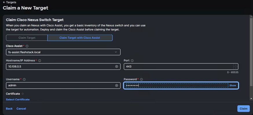
Step 3. Under Admin, click Target then click Claim a New Target. Under Categories, select Network, click Cisco Nexus Switch, and then click Start.
Step 4. Select the Cisco Assist name which is already deployed and configured. Provide the Cisco Nexus Switch management IP address, username and password details and click Claim.
Step 5. Repeat steps 1 through 4 to claim the remaining Switch B.
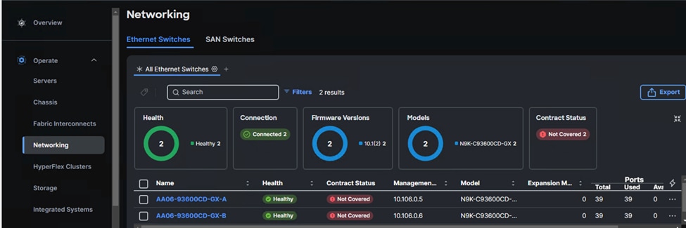
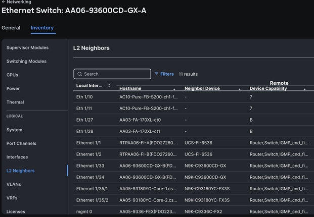
Step 6. When the storage is successfully claimed, from the drop-down list, select Infrastructure Services. Under Operate, click Networking tab. On the right you will find the newly claimed Cisco Nexus switch details and browse through the Switches for viewing the inventory details.
The L2 neighbors of the Cisco Nexus Switch-A is shown below:
Cisco Intersight Managed Mode Configuration for Cisco UCS
The chapter contains the following:
● Fabric Interconnect Domain Profile and Policies
● Server Profile Templates and Policies
● Ethernet Adapter Policy for Storage Traffic
● Compute Configuration Policies
● Management Configuration Policies
The procedures in this chapter describe how to configure a Cisco UCS domain for use in a base FlashStack environment. A Cisco UCS domain is defined as a pair for Cisco UCS FIs and all the servers connected to it. These can be managed using two methods: UCSM and IMM. The procedures detailed below are for Cisco UCS Fabric Interconnects running in Intersight managed mode (IMM).
The Cisco Intersight platform is a management solution delivered as a service with embedded analytics for Cisco and third-party IT infrastructures. The Cisco Intersight Managed Mode (also referred to as Cisco IMM or Intersight Managed Mode) is an architecture that manages Cisco Unified Computing System (Cisco UCS) fabric interconnect–attached systems through a Redfish-based standard model. Cisco Intersight managed mode standardizes both policy and operation management for Cisco UCS C-Series M7 and Cisco UCS X210c M7 compute nodes used in this deployment guide.
Note: This deployment guide assumes an Intersight account is already created, configured with required licenses and ready to use. Intersight Default Resource Group and Default Organizations are used for claiming all the physical components of the FlashStack solution.
Note: This deployment guide assumes that the initial day-0 configuration of Fabric Interconnects is already done in the IMM mode and claimed into the Intersight account.
Procedure 1. Fabric Interconnect Domain Profile and Policies
Step 1. Log into the Intersight portal and select Infrastructure Service. On the left select Profiles then under Profiles select UCS Domain Profiles.
Step 2. Click Create UCS Domain Profile to create a new domain profile for Fabric Interconnects. Under the General tab, select the Default Organization, enter name and descriptions of the profile.
Step 3. Click Next to go to UCS Domain Assignment. Click Assign Later.
Step 4. Click Next to go to VLAN & VSAN Configuration.
Step 5. Under VLAN & VSAN Configuration > VLAN Configuration, click Select Policy then click Create New.
Step 6. On the Create VLAN page, go to the General tab, enter a name (AA06-FI-VLANs), and click Next to go to Policy Details.
Step 7. To add a VLAN, click Add VLANs.
Step 8. For the Prefix, enter the VLAN name as OOB-Mgmt-VLAN. For the VLAN ID, enter the VLAN ID 1061. Leave Auto Allow on Uplinks enabled and Enable VLAN Sharing disabled.
Step 9. Under Multicast Policy, click Select Policy and select Create New to create a Multicast policy.
Step 10. On the Create Multicast Policy page, enter the name (AA06-FI-MultiCast) of the policy and click Next to go to Policy Details. Leave the Snooping State and Source IP Proxy state checked/enabled and click Create. Select the newly created Multicast policy.
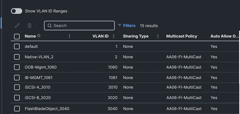
Step 11. Repeat steps 1 through 10 to add all the required VLANs to the VLAN policy.
Step 12. After adding all the VLANs, click Set Native VLAN ID and enter the native VLANs (for example 2) and click Create. The VLANs used for this solution are shown below:
Step 13. Select the newly created VLAN policy for both Fabric Interconnects A and B. Click Next to go to Port Configuration.
Step 14. Enter the name of the policy (AA06-FI-PortConfig) and click Next then click Next again to go to Port Roles Page.
Step 15. In the right pane, under ports, select port 1 and 2 and click Configure.
Step 16. Set Role as Server and leave Auto Negotiation enabled and click Save.
Step 17. In the right pane click the Port Channel tab and click Create Port Channel.
Step 18. For the Role, select Ethernet Uplink Port Channel. Enter 201 as Port Channel ID. Set Admin speed as 100Gbps and FEC as Cl91.
Step 19. Under Link Control, create a new link control policy with the following options. Once created, select the policy.
| Policy Name |
Setting Name |
| AA06-FI-LinkControll
|
UDLD Admin State: True UDLD mode: Normal |
Step 20. For the Uplink Port Channel select Ports 1 and 2 and click Create to complete the Port Roles policy.
Step 21. Click Next to go to UCS Domain Configuration page.
Table 6 lists the Management and Network related policies that are created and used.
| Policy Name |
Setting Name |
| AA06-FI-OCP-NTP
|
Enable ntp: on Server list: 172.20.10.11,172.20.10.12,172.20.10.13 Timezone: America/New_York |
Table 7. Network Connectivity Policy
| Policy Name |
Setting Name |
| AA06-FS-OCP-NWPolicy
|
Proffered IPV4 DNS Server: 10.106.1.21 Alternate IPV4 DNS Server: 10.106.1.22 |
| Policy Name |
Setting Name |
| AA06-FS-OCP-SNMP
|
Enable SNMP: On (select Both v2c and v3) Snmp Port: 161 System Contact: your snmp admin email address System location: Location details snmp user: Name: snmpadmin Security level: AuthPriv Set Auth and Privacy passwords. |
| Policy Name |
Setting Name |
| AA06-FS-OCP-SystemQoS
|
Best Effort: Enable Weight: 5 MTU: 9216 |
Step 22. When the UCS Domain profile is created with the above mentioned policies, edit the policy and assign it to the Fabric Interconnects.
Intersight will go through the discovery process and discover all the Cisco UCS C and X -Series compute nodes attached to the Fabric Interconnects.
Procedure 2. Server Profile Templates and Policies
In the Cisco Intersight platform, a server profile enables resource management by simplifying policy alignment and server configuration. The server profiles are derived from a server profile template. A Server profile template and its associated policies can be created using the server profile template wizard. After creating the server profile template, you can derive multiple consistent server profiles from the template.
The server profile templates captured in this deployment guide supports Cisco UCS X210c M7 compute nodes with 5th Generation VICs and can be modified to support other Cisco UCS blades and rack mount servers.
The following pools need to be created before proceeding with server profile template creation.
MAC Pools
Table 10 lists the two MAC pools for the vNICs that will be configured in the templates.
Table 10. MAC Pool Names and Address Ranges
| MAC Pool Name |
Address Ranges |
| AA06-OCP-IB-MGMT-IPPool-A |
From: 00:25:B5:A6:0A:00 Size: 64 |
| AA06-OCP-IB-MGMT-IPPool-B |
From: 00:25:B5:A6:0B:00 Size: 64 |
UUID pool
Table 11 lists the settings for the UUID pools.
Table 11. UUID Pool Names and Settings
| UUID Pool Name |
Settings |
| AA06-OCP-UUIDPool |
UUID Prefix: AA060000-0000-0001 From: AA06-000000000001 To: AA06-000000000080 Size: 128 |
| AA06-OCP-IB-MGMT-IPPool-B |
From: 00:25:B5:A6:0B:00 Size: 64 |
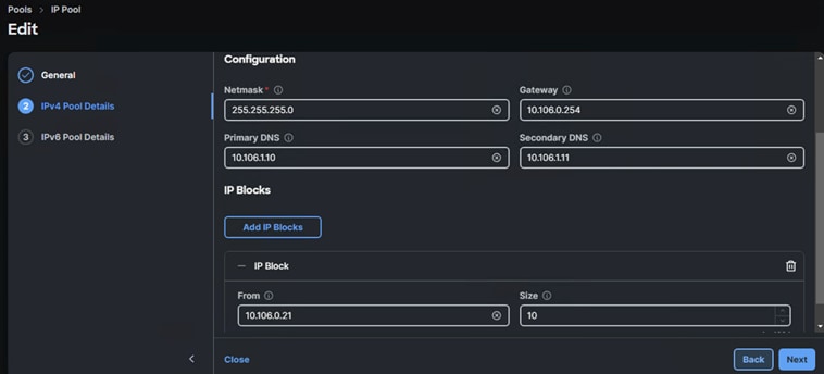
Out-Of-Band (OOB) Management IP Pool
A OOB management IP pool (AA06-OCP-OOB-MGMT-IPPool) is created with following settings:
In this deployment, separate server profile templates are created for Worker and Master Nodes where Worker Nodes have storage network interfaces to support workloads, but Master Nodes do not. The vNIC layout is explained below. While most of the policies are common across various templates, the LAN connectivity policies are unique and use the information in the tables below.
The following vNIC templates are used for deriving the vNICs for OpenShift worker nodes for host management, VM management and iSCSI storage traffics.
Table 12. vNIC Templates for Ethernet Traffic
| Template Name |
AA06-OCP-Mgmt-vNIC Template |
AA06-OCP-iSCSIA-vNIC Template |
AA06-OCP-iSCSIB-vNIC Template |
AA06-OCP-ObjStorage vNIC Template |
| Purpose
|
Carries In-Band management of OpenShift hosts |
Carries iSCSI traffic through fabric-A |
Carries iSCSI traffic through fabric-B |
Carries Object storage of workers nodes |
| Mac Pool |
AA06-OCP-MACPool-A |
AA06-OCP-MACPool-A |
AA06-OCP-MACPool-B |
AA06-OCP-MACPool-B |
| Switch ID |
A |
A |
B |
B |
| CDN Source setting |
vNIC Name |
vNIC Name |
vNIC Name |
vNIC Name |
| Fabric Failover setting |
Yes |
No |
No |
Yes |
| Network Group Policy name and Allowed VLANs and Native VLAN |
AA06-OCP-BareMetal-NetGrp : Native and Allowed VLAN: 1061 |
AA06-OCP-iSCSI-A-NetGrp: Native and Allowed VLAN: 3010 |
AA06-OCP-iSCSIB-NetGrp: Native and Allowed VLAN: 3020 |
AA06-OCP- ObjectStore_NetGrp |
| Network Control Policy Name and CDP and LLDP settings |
AA06-OCP-CDPLLDP: CDP Enabled LLDP (Tx and Rx) Enable |
AA06-OCP-CDPLLDP: CDP Enabled LLDP (Tx and Rx) Enable |
AA06-OCP-CDPLLDP: CDP Enabled LLDP (Tx and Rx) Enable |
AA06-OCP-CDPLLDP: CDP Enabled LLDP (Tx and Rx) Enable |
| QoS Policy name and Settings |
AA06-OCP-MTU1500-MgmtQoS: Best Effort MTU: 1500 Rate Limit (Mbps): 100000 |
AA06-OCP-iSCSI-QoS: Best-effort MTU:9000 Rate Limit (Mbps): 100000 |
AA06-OCP-iSCSI-QoS: Best-effort MTU:9000 Rate Limit (Mbps): 100000 |
AA06-OCP-iSCSI-QoS: Best Effort MTU: 9000 Rate Limit (Mbps): 100000 |
| Ethernet Adapter Policy Name and Settings |
AA06-OCP-EthAdapter-Linux-v2: Uses system defined Policy: Linux-V2 |
AA06-OCP-EthAdapter-16RXQs-5G (refer below section) |
AA06-OCP-EthAdapter-16RXQs-5G (refer below section) |
AA06-OCP-EthAdapter-16RXQs-5G (refer below section) |
Ethernet Adapter Policy for Storage Traffic
The ethernet adapter policy is used to set the interrupts, send and receive queues, and queue ring size. The values are set according to the best-practices guidance for the operating system in use. Cisco Intersight provides a default Linux Ethernet Adapter policy for typical Linux deployments.
You can optionally configure a tweaked ethernet adapter policy for additional hardware receive queues handled by multiple CPUs in scenarios where there is a lot of traffic and multiple flows. In this deployment, a modified ethernet adapter policy, AA06-EthAdapter-16RXQs-5G, is created and attached to storage vNICs. Non-storage vNICs will use the default Linux-v2 Ethernet Adapter policy. Table 13 lists the settings that are changed from defaults in the Adapter policy used for the iSCSI traffic. The remaining settings are left at defaults.
| Setting Name |
Value |
| Name of the Policy |
AA06-OCP-EthAdapter-16RXQs-5G |
| Interrupt Settings |
Interrupts: 19, Interrupt Mode: MSX ,Interrupt Timer: 125 |
| Receive |
Receive Queue Count: 16, Receive Ring Size: 16384 |
| Transmit |
Transmit Queue Count: 1, Transmit Ring Size: 16384 |
| Completion |
Completion Queue Count: 17, Completion Ring Size: 1 |
Using the templates listed in Table 12, separate LAN connectivity policies are created for control and worker nodes.
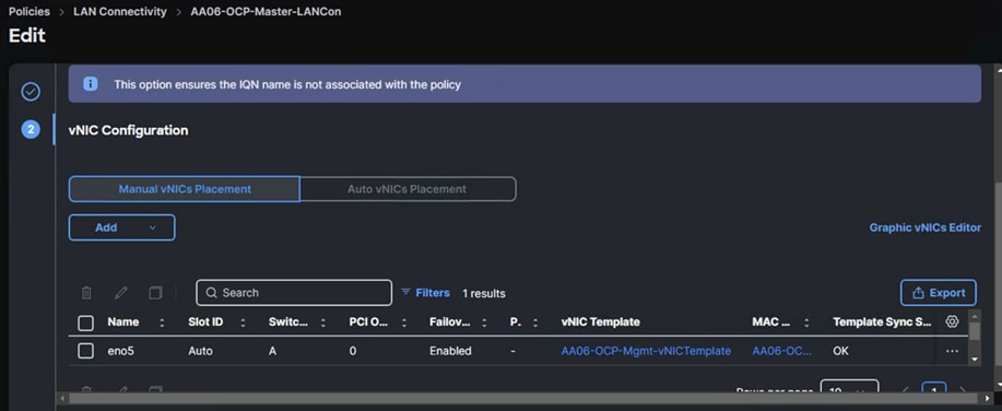
Control nodes are configured with one vNIC which is derived from the AA06-OCP-Mgmt-vNIC template. The following screenshot shows the LAN connectivity policy (AA06-OCP-master-LANCon) created with one vNIC for control node.
Worker nodes are configured with four vNICs which are derived from the templates discussed above. Following screenshot shows the LAN connectivity policy (AA06-OCP-Worker-LANConn) created with four vNICs for worker nodes.
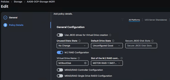
For this solution, Cisco UCS X210c nodes are configured to boot from local M.2 SSD disks. Two M.2 disks are used and configured with RAID-1 configuration. Boot from SAN option will be supported in the next releases. The following screenshot shows the storage policy (AA06-OCP-Storage-M2R1), and the settings used for configuring the M.2 disks in RAID-1 mode.
Compute Configuration Policies
Boot Policy
To facilitate the automatic boot from the Red Hat CoreOS Discovery ISO image, CIMC Mapped DVD boot option is used. The following boot policy is used for both controller and workers nodes.
Note: It is critical to not enable UEFI Secure Boot. Secure Boot needs to be disabled for the proper functionality of Portworx Enterprise and the NVIDIA GPU Operator GPU driver initialization.
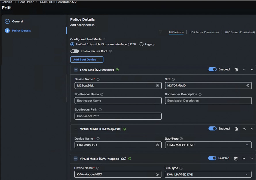
Local Disk boot option being at the top ensures that the nodes always boot from the M.2 disks once after CoreOS installed. The CIMC Mapped DVC option at the second is used to install the CoreOS using Discovery ISO which is mapped using a Virtual Media policy (CIMCMap-ISO). KVM Mapped DVD will be used if you want to manually mount any ISO to the KVM session of the server and install the OS. This option will be used when installing CoreOS during the OpenShift cluster expansion by adding additional worker node.
Virtual Media (vMedia) Policy
Virtual Media policy is used to mount the Red Hat CoreOS Discovery ISO to the server using CIMC Mapped DVD policy as previously explained. A file share service is required to be configured and must be accessed by OOB-Mgmt network. In this solution, the HTTP file share service is used to share the Discovery ISO over the network.
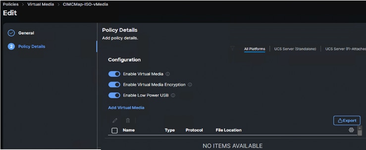
Note: Do not Add Virtual Media at this time, but the policy can be modified later and used to map an OpenShift Discovery ISO to a CIMC Mapped DVD policy.
Procedure 1. Bios Policy
Note: For the OpenShift containerized and Virtualized solution, which is based on Intel M7 platform, the system defined “virtualization-M7-Intel” policy is used in this solution.
Step 1. Create the BIOS policy and select the pre-defined policy as shown below and click Next.
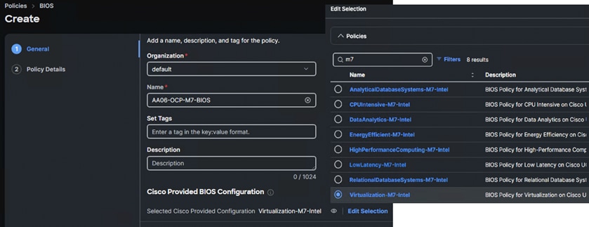
Step 2. Expand Server Management and set Consistent Device Name (CDN) to enabled for Consistent Device Naming within the Operating System.
Note: The remaining bios tokens and their values mentioned are based on the best practices guide from the M7 platform. For more details, go to: Performance Tuning Best Practices Guide for Cisco UCS M7 Platforms.
Step 3. Click Create to complete the BIOS policy.
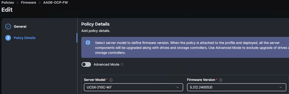
Procedure 2. Firmware Policy (optional)
Step 1. Create a Firmware policy (AA06-OCP-FW) and under the Policy Detail tab, set the Server Model as UCSX-210C-M7 and set Firmware Version to the latest version. The following screenshot shows the firmware policy used in this solution:
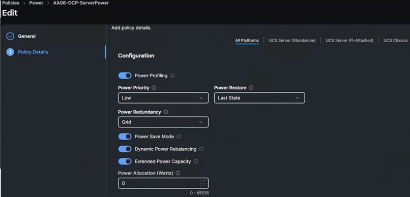
Procedure 3. Create a Power Policy
Step 1. Select All Platform (unless you want to create a dedicated power policy for FI-Attached servers). Select the following options and leave the rest of the settings at default. When you apply this policy to the server profile template, the system will take appropriate settings and apply to the server.
Management Configuration Policies
The following policies will be added to the management configuration:
● IMC Access to define the pool of IP addresses for compute node KVM access
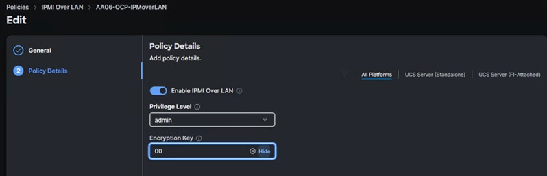
● IPMI Over LAN to allow the servers to be managed by IPMI or redfish through the BMC or CIMC
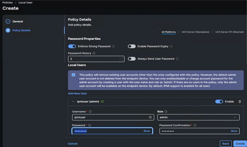
● Local User to provide local administrator to access KVM
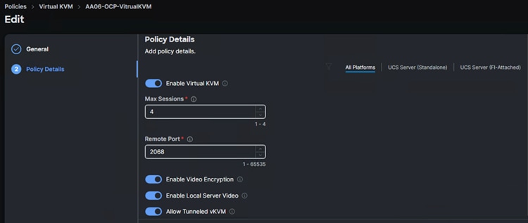
● Virtual KVM to allow the Tunneled KVM
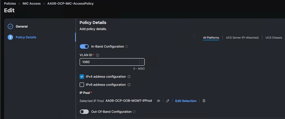
Cisco IMC Access Policy
Create a CIMC Access Policy with settings as shown in the following screenshot.
Note: Since certain features are not yet enabled for Out-of-Band Configuration (accessed using the Fabric Interconnect mgmt0 ports), you need to access the OOB-MGMT VLAN (1060) through the Fabric Interconnect Uplinks and mapping it as the In-Band Configuration VLAN.
IPMI over LAN and Local User Policies
The IPMI Over LAN Policy can be used to allow both IPMI and Redfish connectivity to Cisco UCS Servers. Red Hat OpenShift platform uses these two policies to power manage (power off, restart, and so on) the baremetal servers.
Create the IPMI over LAN policy (AA06-IPMIOvelLan) as shown below:
Virtual KVM Policy
The following screenshot shows the virtual KVM policy (AA06-OCP-VirtualKVM) used in the solution:
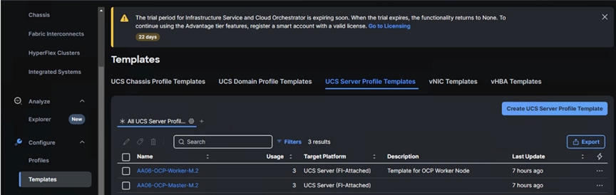
Create Server Profile Templates
When you have the required pools, polices, vNIC templates created, Server profile templates can be created. Two separate Server Profile Templates are used for control and workers node.
Table 14 lists the polices and pools used to create the Server Profile template (AA06-OCP-Master-M.2) for Control nodes.
Table 14. Policies and Pools for Control Nodes
| Page Name |
Setting |
| General |
Name: AA06-OCP-Master-M.2 |
| Compute Configuration |
UUID: AA06-OCP-UUIDPool BIOS: AA06-OCP-M7-BIOS Boot Order: AA06-OCP-BootOrder-M2 Firmware: AA06-OCP-FW Power: AA06-OCP-ServerPower Virtual Media: CIMCMap-ISO-vMedia |
| Management Configuration: |
IMC Access: AA06-OCP-IMC-AccessPolicy IPMI Over LAN: AA06-OCP-IPMoverLAN Local User: AA06-OCP-IMCLocalUser Virtual KVM: AA06-OCP-VitrualKVM |
| Storage Configuration |
Storage: AA06-OCP-Storage-M2R1 |
| Network Configuration |
LAN Connectivity: AA06-OCP-Master-LANCon |
Table 15 lists the polices and pools used to create the Server Profile template (AA06-OCP-Worker-M.2) for worker nodes.
Table 15. Policies and Pools for Worder Nodes
| Page Name |
Setting |
| General
|
Name: AA06-OCP-Worker-M.2 |
| Compute Configuration |
UUID: AA06-OCP-UUIDPool BIOS: AA06-OCP-M7-BIOS Boot Order: AA06-OCP-BootOrder-M2 Firmware: AA06-OCP-FW Power: AA06-OCP-ServerPower Virtual Media: CIMCMap-ISO-vMedia |
| Management Configuration: |
IMC Access: AA06-OCP-IMC-AccessPolicy IPMI Over LAN: AA06-OCP-IPMoverLAN Local User: AA06-OCP-IMCLocalUser Virtual KVM: AA06-OCP-VitrualKVM |
| Storage Configuration |
Storage: AA06-OCP-Storage-M2R1
|
| Network Configuration |
LAN Connectivity: AA06-OCP-Worker-LANConn |
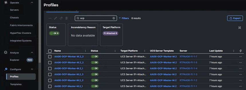
The following screenshot shows the two server profile templates created for the control and worker nodes:
Create Server Profiles
Once Server Profile Templates are created, the server profiles can be derived from the template. The following screenshot shows a total of six profiles are derived (three for control nodes and three for worker nodes).
When the Server profiles are created, associate these server profiles to the control and workers nodes as shown below:
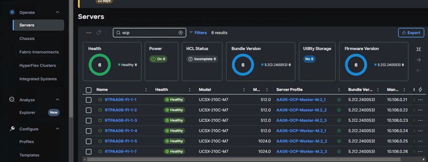
Now the Cisco UCS X210c M7 blades are ready and OpenShift can be installed on these machines.
Pure Storage FlashArray Configuration
This chapter contains the following:
● Claim Pure Storage FlashArray//XL170 into Intersight
In this solution, Pure Storage FlashArray//XL170 is used as the storage provider for all the application pods and virtual machines provisioned on the OpenShift cluster using Portworx Enterprise. The Pure Storage FlashArray//XL170 array will be used as Cloud Storage Provider for Portworx which allows us to store data on-premises with FlashArray while benefiting from Portworx Enterprise cloud drive features.
This chapter describes the high-level steps to configure Pure Storage FlashArray//X170 network interfaces required for storage connectivity over iSCSI. For this solution, Pure Storage FlashArray was loaded with Purity//FA Version 6.6.10.
Note: This document is not intended to explain every day-0 initial configuration steps to bring the array up and running. For detailed day-0 configuration steps, see: https://www.cisco.com/c/en/us/td/docs/unified_computing/ucs/UCS_CVDs/flashstack_ucs_xseries_e2e_5gen.html#FlashArrayConfiguration
The compute nodes are redundantly connected to the storage controllers through 4 x 100Gb connections (2 x 100Gb per storage controller module) from the redundant Cisco Nexus switches.
The Pure Storage FlashArray network settings were configured with three subnets across three VLANs. Storage Interfaces CT0.Eth0 and CT1.Eth0 were configured to access management for the storage on VLAN 1063. Storage Interfaces (CT0.Eth18, CT0.Eth19, CT1.Eth18, and CT1.Eth19) were configured to run iSCSI Storage network traffic on the VLAN 3010 and VLAN 3020.
The following tables provide the IP addressing configured on the interfaces used for storage access.
Table 16. iSCSI A Pure Storage FlashArray//XL170 Interface Configuration Settings
| FlashArray Controller |
iSCSI Port |
IP Address |
Subnet |
| FlashArray//X170 Controller 0 |
CT0.ETH18 |
192.168.51.4 |
255.255.255.0 |
| FlashArray//X170 Controller 1 |
CT1.ETH18 |
192.168.51.5 |
255.255.255.0 |
Table 17. iSCSI B Pure Storage FlashArray//XL170 Interface Configuration Settings
| FlashArray Controller |
iSCSI Port |
IP Address |
Subnet |
| FlashArray//X170 Controller 0 |
CT0.ETH19 |
192.168.52.4 |
255.255.255.0 |
| FlashArray//X170 Controller 1 |
CT1.ETH19 |
192.168.52.5 |
255.255.255.0 |
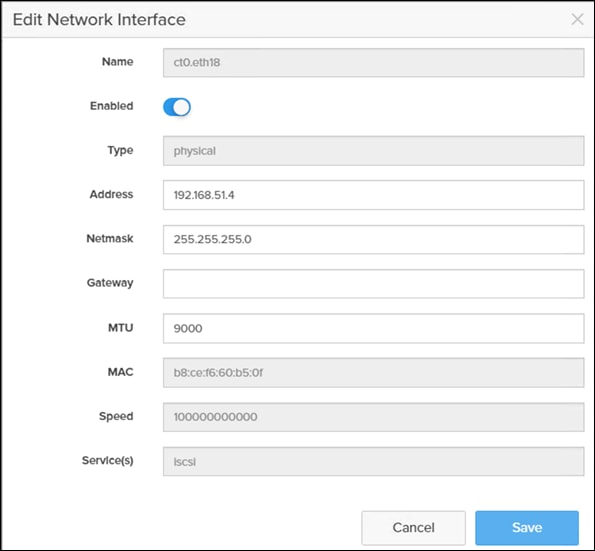
Procedure 1. Configure iSCSI Interfaces
Step 1. Log into Pure FlashArray//XL170 using its management IP addresses.
Step 2. Click Settings > Network > Connectors > Ethernet.
Step 3. Click Edit for Interface CT0.eth18.
Step 4. Click Enable and add the IP information from Table 16 and Table 17 and set the MTU to 9000.
Step 5. Click Save.
Step 6. Repeat steps 1 through 5 to configure the remaining interfaces CT0.eth19, CT1.eth18 and CT1.eth19.
Procedure 2. Claim Pure Storage FlashArray//XL170 into Intersight
Note: This procedure assumes that Cisco Intersight is already hosted outside the OpenShift cluster and Pure Storage FlashArray//XL170 is claimed into the Intersight.com.
Step 1. Log into Cisco Intersight using your login credentials. From the drop-down menu select System.
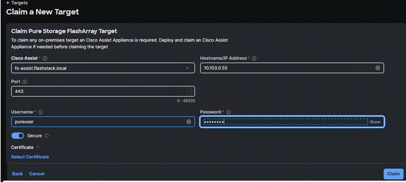
Step 2. Under Admin, select Target and click Claim a New Target. Under Categories, select Storage, click Pure Storage FlashArray and then click Start.
Step 3. Select the Cisco Assist name which is already deployed and configured. Provide the Pure Storage FlashArray management IP address, username, and password details and click Claim.
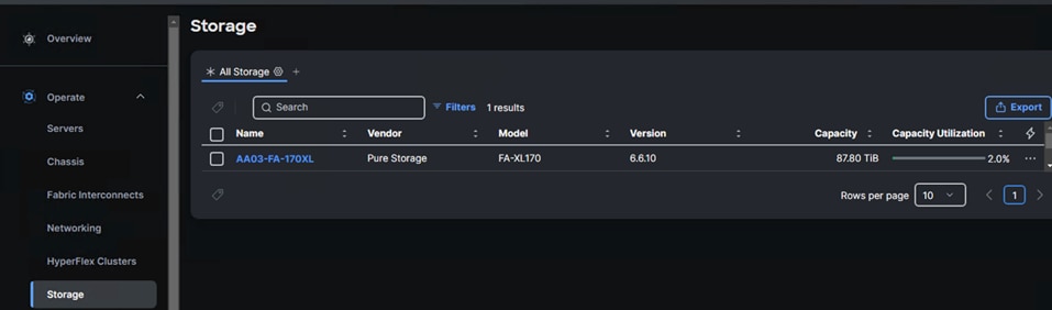
Step 4. When the storage is successfully claimed, from the drop-down list, select Infrastructure Services. Under Operate, click Storage. You will see the newly claimed Pure Storage FlashArray; browse through it to view the inventory details.
Pure Storage FlashBlade Configuration
This chapter contains the following:
In this solution, Pure Storage FlashBlade//S200 is used as the persistent object storage provider for the Milvus vector database hosted on the OpenShift cluster. The FlashBlade is directly accessed by the Milvus vector database pod by using Workers node’s interface that carries object storage traffic (eno8). This section describes high-level steps to configure Pure Storage FlashBlade//S200 network interfaces required for storage connectivity over ethernet. Pure Storage FlashBlade was loaded with Purity//FB V4.1.12.
The FlashBlade//S200 provides up to 8x 100GbE interfaces for data traffic. In this solution, 2x 100GbE from each FIOM (with aggregated network bandwidth of 400 GbE) are connected to a pair of Nexus switches. For more details about FlashBlade connectivity, see section Pure Storage FlashBlade//S200 Ethernet Connectivity.
Note: This document is not intended to explain every day-0 initial configuration steps to bring the array up and running. For day-0 configuration steps, see: https://support.purestorage.com/bundle/m_flashblades/page/FlashBlade/FlashBlade_Hardware/topics/concept/c_flashblades.html
Table 18 provides the IP addressing configured on the interfaces used for objects storage access.
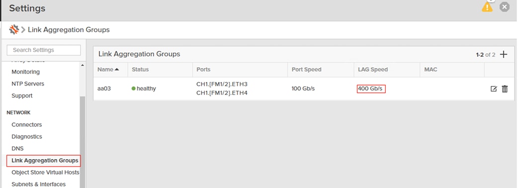
Table 18. Link Aggregation Groups (LAG)
| LAG Name |
FM |
Ethernet Ports |
| AA03
|
1 |
CH1. FM1.ETH3 & CH1. FM1.ETH4 |
| 2 |
CH1. FM2.ETH3 & CH1. FM2.ETH4 |
A Link Aggregation Group is created using CH1.FM1.ETH3, CH1.FM1.ETH4, CH1.FM2.ETH3, and CH1.FM2.ETH4 interfaces as shown below. Notice that the aggregated bandwidth of the LAG is 400GbE as it is created with 4x 100GbE interfaces as shown below:
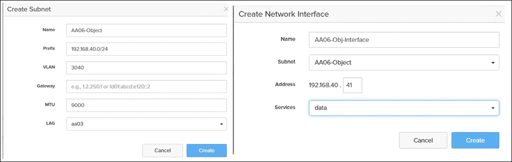
Once the LAG is created, a Subnet (AA06-Object) and an interface (AA06-Obj-Interface) is created as shown below. For the subnet, ensure to set MTU as 9000, VLAN as 3040 and select “aa03” for the LAG. Ensure to set Services as “Data” for the interface.
FlashBlade Object Store configuration involves creating an Object Store Account, user, Access Keys and finally a bucket.
Procedure 1. Create a Object Store Account, User, Access Keys and Bucket
Step 1. Log into Pure FlashBlade//S200 using its management IP addresses.
Step 2. Click Storage > Object Store > Accounts > Click + to create an account.
Step 3. Provide a name for Account, Quota Limit and Bucket Default Quota Limit as per your requirements. Click on Create.
Step 4. Click the newly created Account name and click + to create a new user for the account.
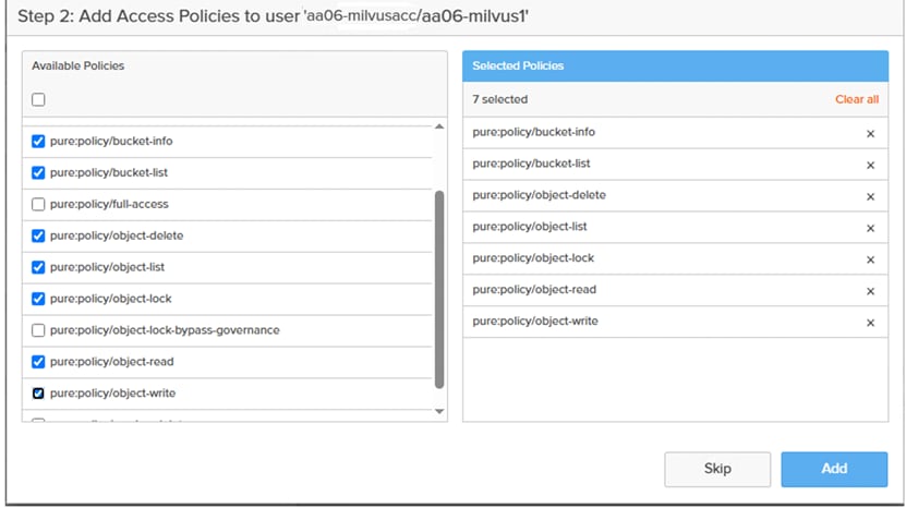
Step 5. Provide a username and click Create.
Step 6. In the Add Access Policies window, select the pre-defined access policies as shown below. Or create your own access policy with a set of rules and finally select it.
Step 7. Click Add when Access Policy is selected.
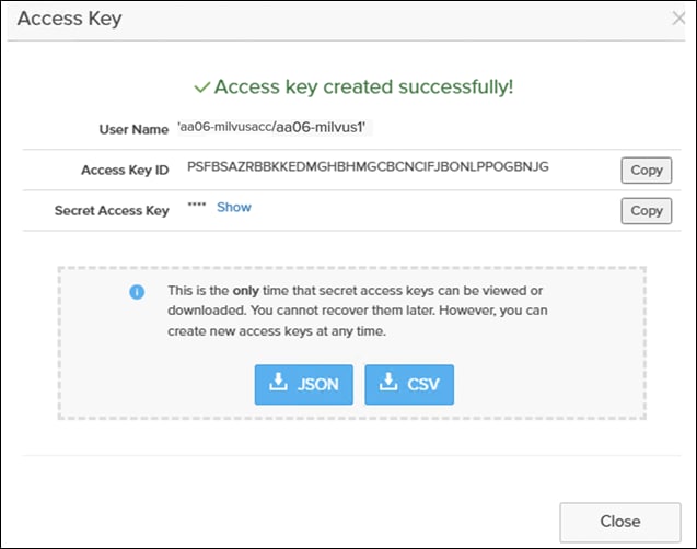
Step 8. Click Create a new key and click Create to create a pair of access and secret keys. Preserve the Access and Secret Keys for later use. Click Close.
Step 9. Click Account name and go to the Buckets sections. Click + to create a bucket and add it to the account.
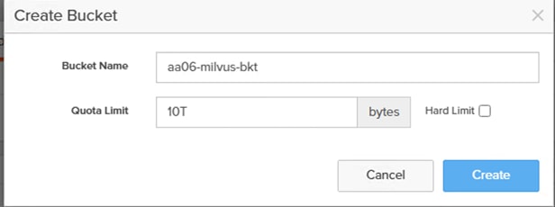
Step 10. Provide a bucket name and Quota Limit. Click Create.
This completes the FlashBlade configuration for object store access by the Milvus vector database pods.
OpenShift Container Platform Installation and Configuration
This chapter contains the following:
● OpenShift Container Platform – Installation Requirements
OpenShift 4.16 is deployed on the Cisco UCS infrastructure as M.2 booted bare metal servers. The Cisco UCS X210C M7 servers need to be equipped with an M.2 controller (SATA or NVMe) card and two identical M.2 drives. Three master nodes and three worker nodes are deployed in the validation environment and additional worker nodes can easily be added to increase the scalability of the solution. This document will guide you through the process of using the Assisted Installer to deploy OpenShift 4.17.
OpenShift Container Platform – Installation Requirements
The Red Hat OpenShift Assisted Installer provides support for installing OpenShift Container Platform on bare metal nodes. This guide provides a methodology to achieving a successful installation using the Assisted Installer.
Prerequisites
The FlashStack for OpenShift utilizes the Assisted Installer for OpenShift installation. Therefore, when provisioning and managing the FlashStack infrastructure, you must provide all the supporting cluster infrastructure and resources, including an installer VM or host, networking, storage, and individual cluster machines.
The following supporting cluster resources are required for the Assisted Installer installation:
● The control plane and compute machines that make up the cluster
● Cluster networking
● Storage for the cluster infrastructure and applications
● The Installer VM or Host
The following infrastructure services need to be deployed to support the OpenShift cluster, during the validation of this solution we have provided VMs on your hypervisor of choice to run the required services. You can use the existing DNS and DHCP services available in the data center.
There are various infrastructure services prerequisites for deploying OpenShift 4.17. These prerequisites are as follows:
● DNS and DHCP services – these services were configured on Microsoft Windows Server VMs in this validation
● NTP Distribution was done with Nexus switches
● Specific DNS entries for deploying OpenShift – added to the DNS server
● A Linux VM for initial automated installation and cluster management – a Rocky Linux / RHEL VM with appropriate packages
NTP
Each OpenShift Container Platform node in the cluster must have access to at least two NTP servers.
NICs
NICs configured on the Cisco UCS servers based on the design previously discussed.
DNS
Clients access the OpenShift Container Platform cluster nodes over the bare metal network. Configure a subdomain or subzone where the canonical name extension is the cluster name.
The following domain and OpenShift cluster names are used in this deployment guide:
● Base Domain: flashstack.local
● OpenShift Cluster Name: fs-ocp1
The DNS domain name for the OpenShift cluster should be the cluster name followed by the base domain, for example fs-ocp1. flashstack.local.
Table 19 lists the information for fully qualified domain names used during validation. The API and Nameserver addresses begin with canonical name extensions. The hostnames of the control plane and worker nodes are exemplary, so you can use any host naming convention you prefer.
| Usage |
Hostname |
IP Address |
| API |
api.fs-ocp1.flashstack.local |
10.106.1.31 |
| Ingress LB (apps) |
*.apps.fs-ocp1.flashstack.local |
10.106.1.32 |
| master1 |
master1.fs-ocp1.flashstack.local |
10.106.1.33 |
| master2 |
master2.fs-ocp1.flashstack.local |
10.106.1.34 |
| master3 |
master3.fs-ocp1.flashstack.local |
10.106.1.35 |
| worker1 |
worker1.fs-ocp1.flashstack.local |
10.106.1.36 |
| worker2 |
worker2.fs-ocp1.flashstack.local |
10.106.1.37 |
| worker3 |
worker3.fs-ocp1.flashstack.local |
10.106.1.38 |
DHCP
For the bare metal network, a network administrator must reserve several IP addresses, including:
● One IP address for the API endpoint
● One IP address for the wildcard Ingress endpoint
● One IP address for each master node (DHCP server assigns to the node)
● One IP address for each worker node (DHCP server assigns to the node)
Note: Get the MAC addresses of the bare metal Interfaces from the UCS Server Profile for each node to be used in the DHCP configuration to assign reserved IP addresses (reservations) to the nodes. The KVM IP address also needs to be gathered for the master and worker nodes from the server profiles.
Procedure 1. Gather MAC Addresses of Node Bare Metal Interfaces
Step 1. Log into Cisco Intersight.
Step 2. Go to Infrastructure Service > Profiles > UCS Server Profile (for example, AA06-OCP-Worker-M.2_3).
Step 3. In the center pane, go to Inventory > Network Adapters > Network Adapter (for example, UCSX-ML-V5D200G).
Step 4. In the center pane, click Interfaces.
Step 5. Record the MAC address for NIC Interface eno5.
Step 6. Select the General tab and click Identifiers.
Step 7. Record the Management IP assigned from the AA06-OCP-OOB-MGMT-IP Pool.
Table 20 lists the IP addresses used for the OpenShift cluster including bare metal network IPs and UCS KVM Management IPs for IMPI or Redfish access.
Table 20. Host BMC Information
| Hostname |
Management IP Address |
UCS KVM Mgmt. IP Address |
BareMetal MAC Address (eno5) |
| master1.fs-ocp1.flashstack.local |
10.106.1.33 |
10.106.0.21 |
00-25-B5-A6-0A-00 |
| master2.fs-ocp1.flashstack.local |
10.106.1.34 |
10.106.0.22 |
00-25-B5-A6-0A-01 |
| master3.fs-ocp1.flashstack.local |
10.106.1.35 |
10.106.0.23 |
00-25-B5-A6-0A-02 |
| worker1.fs-ocp1.flashstack.local |
10.106.1.36 |
10.106.0.24 |
00-25-B5-A6-0A-03 |
| worker2.fs-ocp1.flashstack.local |
10.106.1.37 |
10.106.0.25 |
00-25-B5-A6-0A-09 |
| worker3.fs-ocp1.flashstack.local |
10.106.1.38 |
10.106.0.26 |
00-25-B5-A6-0A-0B |
Step 8. From Table 20, enter the hostnames, IP addresses, and MAC addresses as reservations in your DHCP and DNS server(s) or configure the DHCP server to dynamically update DNS.
Step 9. You need to pipe VLAN interfaces for all 3 storage VLANs (3010, 3020 and 3040) and 1 management VLANs (1061) into your DHCP server(s) and assign IPs in the storage networks on those interfaces.
Step 10. Create a DHCP scope for each management and storage VLANs with the appropriate subnets.
Step 11. Ensure that the IPs assigned by the scope do not overlap with the already consumed IPs (like FlashArray//XL170 storage iSCSI interface IPs, FlashBlade//S200 interfaces and OpenShift reserved IPs).
Step 12. Enter the nodes in the DNS server or configure the DHCP server to forward entries to the DNS server. For the cluster nodes, create reservations to map the hostnames to the desired IP addresses as shown below:
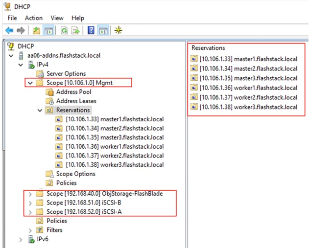
Note: With these DHCP scopes in place, the Management and storage IPs will be assigned automatically from the corresponding DHCP pools to the respective interfaces of master and worker nodes. No manual IP configuration is required.
Step 13. Setup either a VM (installer/bastion node) or spare server with the network interface connected to the Bare Metal VLAN.
Step 14. Install either Red Hat Enterprise Linux (RHEL) 9.4 or Rocky Linux 9.4 Server with GUI and create an administrator user. Once the VM or host is up and running, update it and install and configure XRDP. Connect to this host with a Windows Remote Desktop client as the admin user.
Step 15. ssh into the installer node VM, open a terminal session and create an SSH key pair to use to communicate with the OpenShift hosts:
cd
ssh-keygen -t ed25519 -N '' -f ~/.ssh/id_ed25519
Step 16. Copy the public SSH key to the user directory:
cp ~/.ssh/id_ed25519.pub ~/
Step 17. Add the private key to the ssh-agent:
sshadd ~/.ssh/id_ed25519
Procedure 2. Install Red Hat OpenShift Container Platform using the Assisted Installer
Step 1. Launch Firefox and connect to https://console.redhat.com/openshift/cluster-list. Log into your Red Hat account.
Step 2. Click Create cluster to create an OpenShift cluster.
Step 3. Select Datacenter and then select Bare Metal (x86_64).
Step 4. Select Interactive to launch the Assisted Installer.
Step 5. Provide the cluster name and base domain.
Step 6. Select the latest OpenShift version, scroll down and click Next.
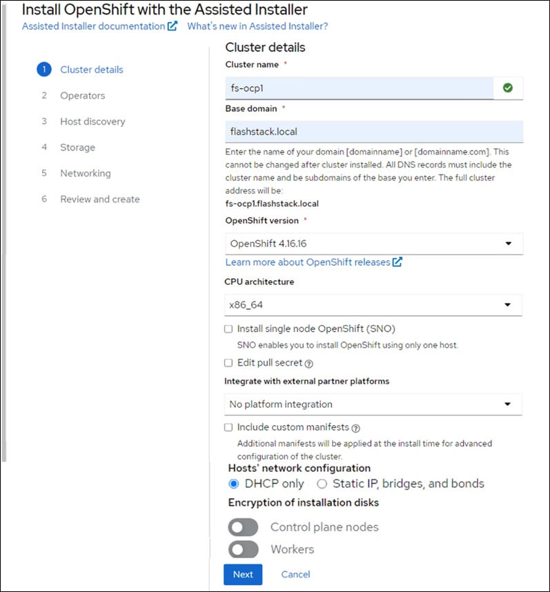
Step 7. Select the latest OpenShift version, scroll down and click Next.
Step 8. Select Install OpenShift Virtualization operator and click Next.
Step 9. Click Add hosts.
Step 10. Under Provisioning type, from the drop-down list select the Full Image file. Under SSH public key, click Browse and browse to, select, and open the id_ed25519.pub file. The contents of the public key should now appear in the box. Click Generate Discovery ISO and click Download Discovery ISO to download the Discovery ISO.

Step 11. Copy the Discovery ISO to a http or https file share server, use a web browser to get a copy of the URL for the Discovery ISO.
Step 12. Log into Cisco Intersight and update the virtual Media policy with the Discovery ISO URL as shown below. This Discovery ISO image will be mapped to the server using CIMC Mapped DVD option defined in the Boot policy.
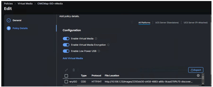
Note: To demonstrate the OpenShift cluster expansion (adding additional worker node), only the first five nodes (3 master/control and 2 workers) will be used for the initial OpenShift cluster deployment. The sixth node is reserved for now and will be used for cluster expansion which will be discussed in the following sections.
Step 13. Go to Operate > Power > Reset System to reset first five UCSX-201c M7 servers.
Step 14. When all five servers have booted RHEL CoreOS (Live) from the Discovery ISO, they will appear in the Assisted Installer. From the drop-down lists under Role assign the appropriate server roles. Scroll down and click Next.
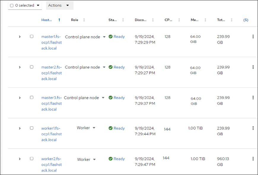
Step 15. Expand each node and confirm the role of the M.2 disk is set to Installation disk. Click Next.
Step 16. Under Network Management, make sure Cluster-Managed Networking is selected. Under Machine network, from the drop-down list, select the subnet for the BareMetal VLAN. Enter the API IP for the api.cluster.basedomain entry in the DNS servers. For the Ingress IP, enter the IP for the *.apps.cluster.basedomain entry in the DNS servers.
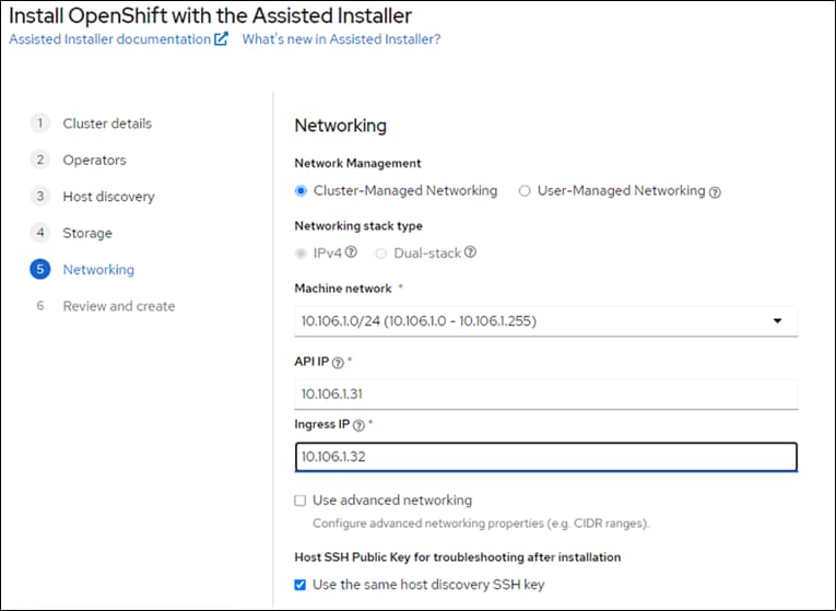
Step 17. Scroll down. All nodes should have a status of Ready.
Note: If you see insufficient warning message for the nodes due to missing ntp server information, expand one of the nodes, click Add NTP Sources and provide the NTP servers IPs separated by a comma.
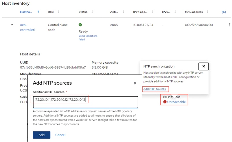
Note: A warning message may display about each worker node having multiple network devices on the L2 network. To resolve this, SSH into each worker and deactivate eno8,eno9, and eno10 interfaces using nmtui utility.
Step 18. When all the nodes are in ready status, click Next.
Step 19. Review the information and click Install cluster to begin the cluster installation.
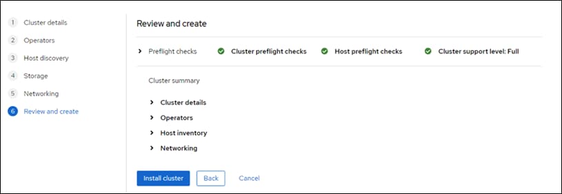
Step 20. On the Installation progress page, expand the Host inventory. The installation will take 30-45 minutes. When the installation is complete, all nodes will show a Status of Installed.
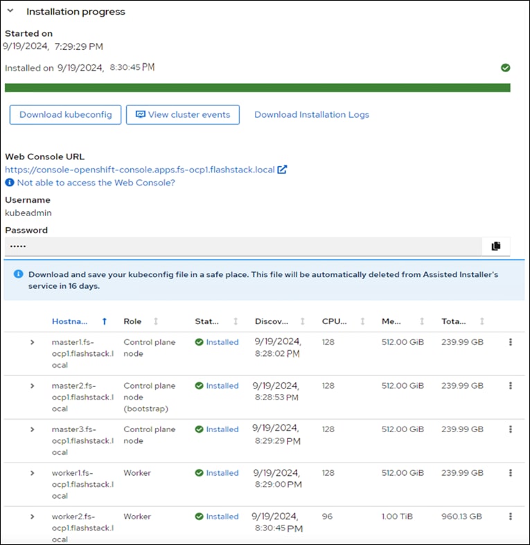
Step 21. Select Download kubeconfig to download the kubeconfig file. In a terminal window, setup a cluster directory and save credentials:
cd
mkdir <clustername> # for example, ocp
cd <clustername>
mkdir auth
cd auth
mv ~/Downloads/kubeconfig ./
mkdir ~/.kube
cp kubeconfig ~/.kube/config
Step 22. In the Assisted Installer, click the icon to copy the kubeadmin password:
echo <paste password> > ./kubeadmin-password
Step 23. Click Open console to launch the OpenShift Console. Log in using the kubeadmin and the kubeadmin password.
Step 24. Click the ? mask. Links for various tools are provided in that page. Download oc for Linux for x86_64 and virtctl for Linux for x86_64 Common Line Tools.
cd ..
mkdir client
cd client
ls ~/Downloads
mv ~/Downloads/oc.tar.gz ./
mv ~/Downloads/virtctl.tar.gz ./
tar xvf oc.tar
tar xvf virtctl.tar.gf
ls
sudo mv oc /usr/local/bin/
sudo mv virtcl /usr/local/bin/
sudo mv kubectl /usr/local/bin/
oc get nodes
Step 25. To enable oc tab completion for bash, run the following:
oc completion bash > oc_bash_completion
sudo mv oc_bash_completion /etc/bash_completion.d/
Step 26. In Cisco Intersight, edit the Virtual Media policy and remove the link to the Discovery ISO.
Step 27. Click Save & Deploy then click Save & Proceed.
Step 28. Do not select “Reboot Immediately to Activate.”
Step 29. Click Deploy. The virtual media mount will be removed from the servers without rebooting them.
Step 30. In Firefox, in the Assisted Installer page, click Open console to launch the OpenShift Console. Log in using the kubeadmin and the kubeadmin password.
Step 31. Go to Compute > Nodes to see the status of the OpenShift nodes.
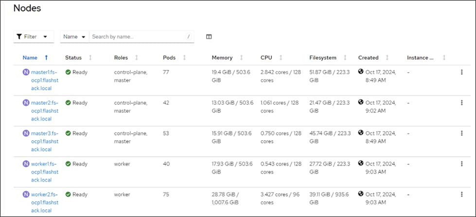
Step 32. In the Red Hat OpenShift console, go to Compute > Bare Metal Hosts. For each Bare Metal Host, click the ellipses to the right of the host and select Edit Bare Metal Host. Select Enable power management.
Step 33. From Table 20, fill in the BMC Address. Also, make sure the Boot MAC Address matches the MAC address in Table 20. For the BMC Username and BMC Password, use what was entered into the Cisco Intersight IPMI over LAN policy. Click Save to save the changes. Repeat this step for all Bare Metal Hosts.
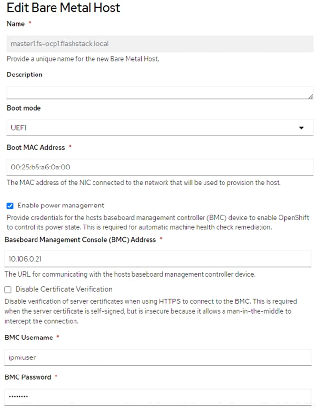
Step 34. Go to Compute > Bare Metal Hosts. When all hosts have been configured, the Status displays “Externally provisioned,” and the Management Address are populated. You can now manage power on the OpenShift hosts from the OpenShift console.
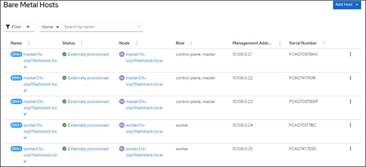
Note: For an IPMI connection to the server, use the BMC IP address. However, for Redfish to connect to the server, use this format for the BMS address; redfish://<BMC IP>/redfish/v1/Systems/<server Serial Number> and make sure to check Disable Certificate Verification. For Instance, for master1.fs-ocp1.flashstack.local Bare Metal node, the redfish BMC management Address will be: redfish://10.106.0.21/redfish/v1/Systems/FCH270978H0. When using Redfish to connect to the server, it is critical to check the box for Disable Certificate Verification.
Note: It is recommended to reserve enough resources (CPU and memory) for system components like kubelet and kube-proxy on the nodes. OpenShift Container Platform can automatically determine the optimal system-reserved CPU and memory resources for nodes associated with a specific machine config pool and update the nodes with those values when the nodes start.
Step 35. To automatically determine and allocate the system-reserved resources on nodes, create a KubeletConfig CUSTOM RESOURCE (CR) to set the autoSizingReserved: true parameter as shown below and apply the machine configuration files:
cat dynamic-resource-alloc-workers.yaml
apiVersion: machineconfiguration.openshift.io/v1
kind: KubeletConfig
metadata:
name: dynamic-node-worker
spec:
autoSizingReserved: true
machineConfigPoolSelector:
matchLabels:
pools.operator.machineconfiguration.openshift.io/worker: ""
cat dynamic-resource-alloc-master.yaml
apiVersion: machineconfiguration.openshift.io/v1
kind: KubeletConfig
metadata:
name: dynamic-resource-allow-master
spec:
autoSizingReserved: true
machineConfigPoolSelector:
matchLabels:
pools.operator.machineconfiguration.openshift.io/master: ""
oc apply -f dynamic-resource-alloc-workers.yaml
oc apply -f dynamic-resource-alloc-master.yaml
Note: To manually configure the resources for the system components on the nodes, go to: https://docs.openshift.com/container-platform/4.16/nodes/nodes/nodes-nodes-resources-configuring.html#nodes-nodes-resources-configuring-setting_nodes-nodes-resources-configuring
Expand OpenShift Cluster by Adding a Worker Node
This chapter contains the following:
● Link the Machine and Bare Metal Host, Node and Bare Metal Host
This chapter provides detailed steps to scale up the worker nodes of OpenShift cluster by adding a new worker node to the existing cluster. For this exercise, the sixth blade in the chassis will be used and be part of the cluster by the end of this exercise.
Note: This chapter assumes that a new server profile is already derived from the existing template and assigned to the new server successfully.
Procedure 1. OpenShift Cluster expansion
Step 1. Launch Firefox and go to https://console.redhat.com/openshift/cluster-list. Log into your Red Hat account.
Step 2. Click your cluster name and go to Add Hosts.
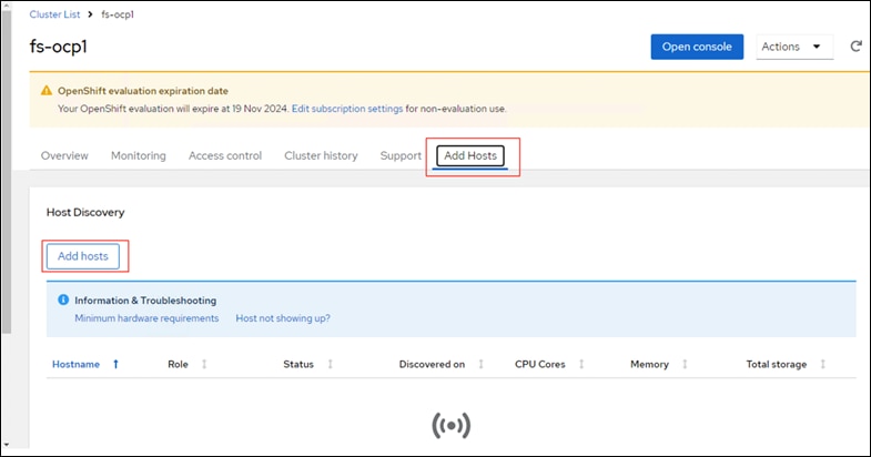
Step 3. Under Host Discovery, click Add hosts.
Step 4. In the Add hosts wizard, for the CPU architecture select x86_64 and for the Host’s network configuration select DHCP Only. Click Next.
Step 5. For the Provision type select Full image file from the drop-down list, for SSH public key browse or copy/paste the contents of id-ed25519.pub file. Click Generate Discovery ISO and when the file is generated and click Download Discovery ISO file.
Step 6. Copy the Discovery ISO to a http or https file share server, use a web browser to get a copy of the URL for the new Discovery ISO.
Step 7. Log into Cisco Intersight and update the virtual Media policy as explained in the previous section. This Discovery ISO image is a mapped server using the CIMC Mapped DVD option. Go to Power > Reset System to reset the sixth UCSX-201c M7 server.
Step 8. When the server has booted “RHEL CoreOS (live)” from the newly generated Discovery ISO, it will appear in the assisted installer under Add hosts.
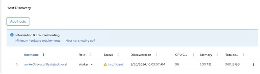
Note: If you see insufficient warning messages for the node due to missing ntp server information, expand one of the nodes, click Add NTP Sources and provide the NTP servers IPs separated by a comma.
Note: If a warning message appears stating you have multiple network devices on the L2 network, ssh into worker node and deactivate eno8,eno9, and eno10 interfaces using the nmtui utility.
Step 9. When the node status shows Ready, click Install ready hosts. After few minutes, the required components will be installed on the node and displays the status as Installed.
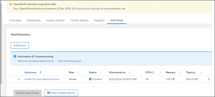
Step 10. When the server successfully produces the CoreOS installed, log into Cisco Intersight, edit the vMedia policy and remove the virtual media mount. Go to Profiles > Server Profiles page, deploy the profile to the newly added worker profile without rebooting the host. The Inconsistent state on the remaining profiles should be cleared.
Step 11. Log into the cluster with kubeadmin user and go to Compute > Nodes > and select the newly added worker node and approve the Cluster join request of the worker node and request for server certificate signing.
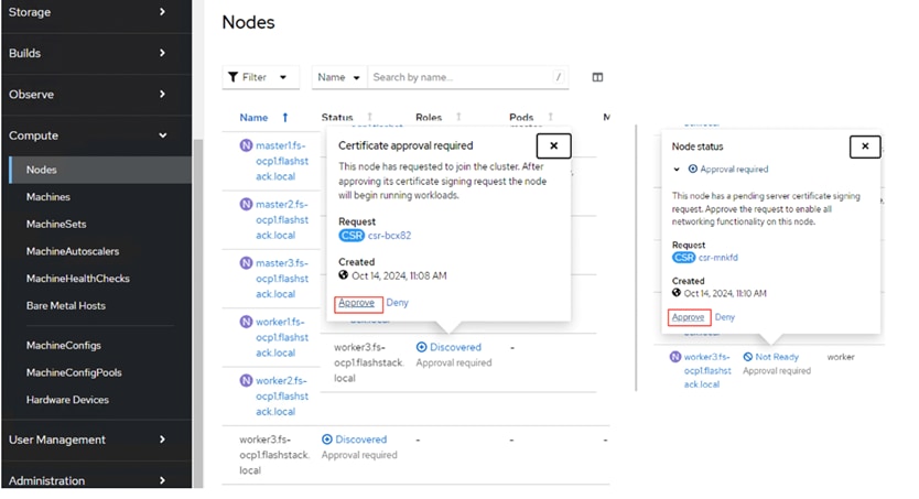
Step 12. Wait for a few seconds and the node will be ready and the pods are scheduled on the newly added worker node.
Step 13. Create secret and BareMetalHost objects in openshift-machine-api namespace by executing the following manifest (bmh-worker3.yaml):
cat bmh-worker3.yaml
---
apiVersion: v1
kind: Secret
metadata:
name: ocp-worker3-bmc-secret
namespace: openshift-machine-api
type: Opaque
data:
username: aXBtaXVzZXIK
password: SDFnaFYwbHQK
---
apiVersion: metal3.io/v1alpha1
kind: BareMetalHost
metadata:
name: worker3.fs-ocp1.flashstack.local
namespace: openshift-machine-api
spec:
online: True
bootMACAddress: 00:25:B5:A6:0A:0B
bmc:
address: redfish://10.106.0.26/redfish/v1/Systems/FCH27477BZU
credentialsName: ocp-worker3-bmc-secret
disableCertificateVerification: True
customDeploy:
method: install_coreos
externallyProvisioned: true
Note: The username and password shown in the above file are base64 encoded values.
Note: In this case, redfish connection is used for connecting to the server. 00:25:B5:A6:0A:0B is the MAC address of eno5 interface, 10.106.0.26 is the OOB management IP and FCH27477BZU is the serial number of the newly added worker node. These values are updated in the table 5. If you would like to use IPMI over LAN instead of redfish, just put the server’s out of band management IP for the bmc address field.
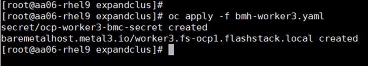
A new entry will be created for the newly added worker node under Compute > Bare Metal Hosts.
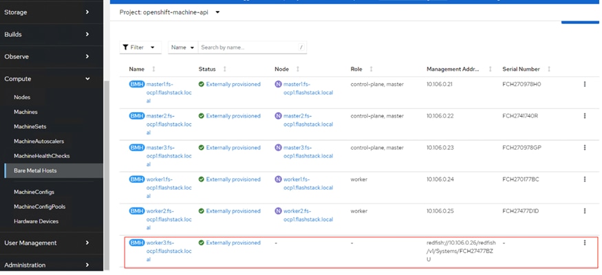
Note: The node field is not yet populated for this bare metal host as it is not yet logically linked to any OpenShift Machine.
Note: Since there are only two machines (workers) in the cluster, the worker MachineSets count needs to be increased from 2 to 3.
Step 14. To increase the worker’s machineset count, go to Compute > MachineSets. Click the ellipses of worker-0 machineset and select Edit Machine Count and increase the count from 2 to 3. Click Save.
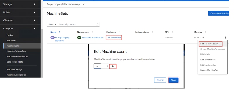
A new worker node will be provisioned to match to the worker machine count of 3. It will be under the provisioning state until the node is logically mapped to the Bare Metal Host.
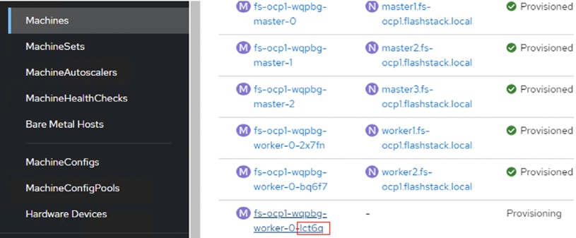
Procedure 2. Link the Machine and Bare Metal Host, Node and Bare Metal Host
Step 1. To logically link Bare Metal Host to Machine, obtain the name of the newly created machine from its manifest file or by executing oc get machine -n openshift-machine-api:
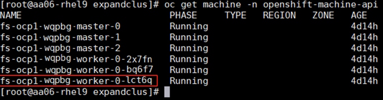
Step 2. Update the machine name in the Bare Metal Host’s manifest file under spec. consumerRef as shown below. Save the Yaml and reload:
consumerRef:
apiVersion: machine.openshift.io/v1beta1
kind: Machine
name: fs-ocp1-wqpbg-worker-0-lct6q
namespace: openshift-machine-api
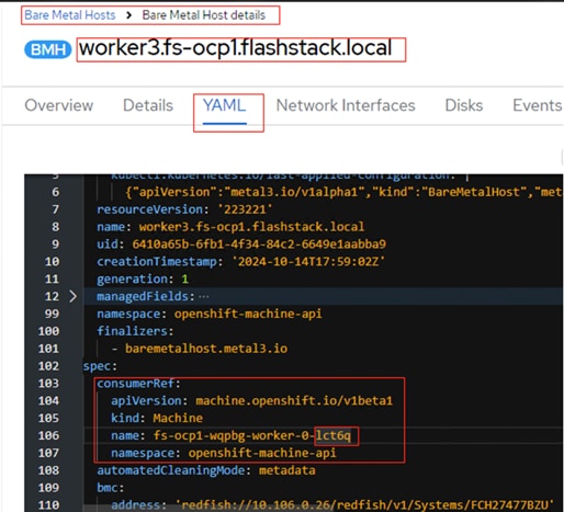
After updating the machine name under Bare Metal Host yaml manifest, the newly created machine will turn to Provisioned as node state from Provisioning state.
Note: The Bare Metal Host ProviderID needs to be generated and updated in the newly added worker (worker3.fs-ocp1.flashstack.local).
The ProviderID is a combination of the name and UUID of the Bare Metal Host and is shown below. These details can be gathered by running providerID: ‘baremetalhost:///openshift-machine-api/<Bare Metal Host Name>/<Bare Metal Host UID>.’
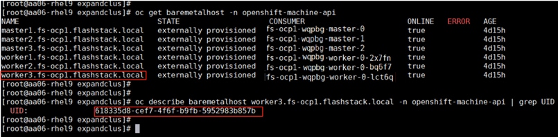
By using the provided information, the providerID for of the newly added Bare Metal Host is built as providerID: ‘baremetalhost:///openshift-machine-api/worker3.fs-ocp1.flashstack.local/6410a65b-6fb1-4f34-84c2-6649e1aabba9.’
Step 3. Copy the providerID of the Bare Metal Host into the third node yaml manifest file under spec. as shown below:
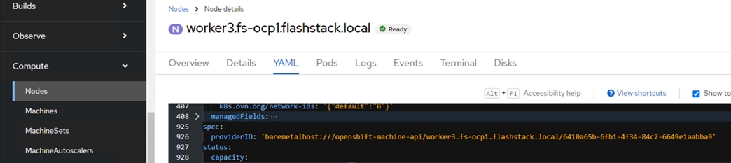
When the providerID of worker3 is updated, the node details are automatically populated for the newly added Bare Metal Host as shown below:
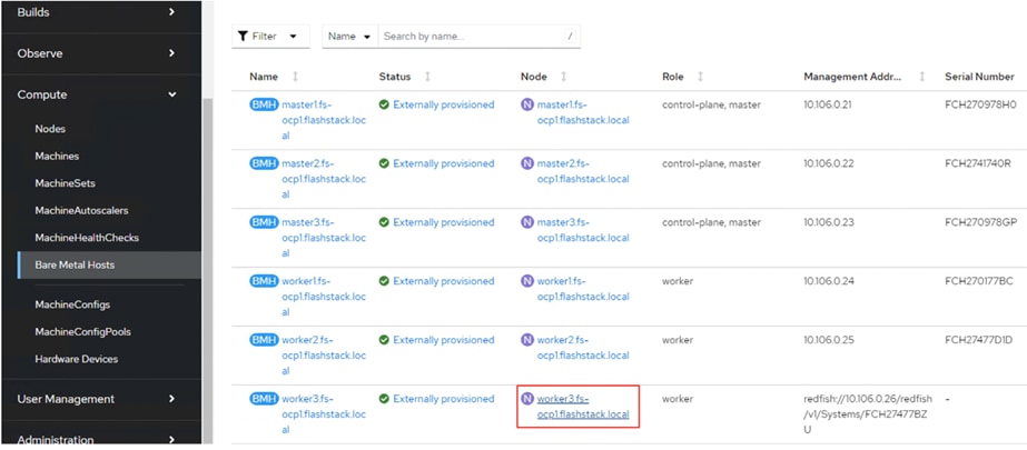
Install NVIDIA GPU Operator and Drivers
This chapter contains the following:
● Enable the GPU Monitoring Dashboard
This chapter provides the procedures to install the required NVIDIA GPU operators, CUDA drivers and so on, to work with NVIDIA GPUs.
Procedure 1. Install NVIDIA GPU Operator
If you have GPUs installed in your Cisco UCS servers, you need to install the Node Feature Discovery (NFD) Operator to detect NVIDIA GPUs and the NVIDIA GPU Operator to make these GPUs available to containers and virtual machines.
Step 1. In the OpenShift Container Platform web console, click Operators > OperatorHub.
Step 2. Type Node Feature in the filter box and then click the Node Feature Discovery Operator with Red Hat in the upper right corner. Click Install.
Step 3. Do not change any settings and click Install.
Step 4. When the Install operator is ready for use, click View Operator.
Step 5. In the bar to the right of Details, click NodeFeatureDiscovery.
Step 6. Click Create NodeFeatureDiscovery.
Step 7. Click Create.
Step 8. When the nfd-instance has a status of Available, Upgradeable, select Compute > Nodes.
Step 9. Select a node that has one or more GPUs and then click Details.
The label feature.node.kubernetes.io/pci-10de.present=true should be present on the host.
This label appears on all nodes with GPUs:
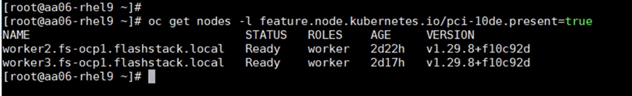
Step 10. Go to Operators > OperatorHub.
Step 11. Type NVIDIA in the filter box and then click the NVIDIA GPU Operator. Click Install.
Step 12. Do not change any settings and click Install.
Step 13. When the Install operator is ready for use, click View Operator.
Step 14. In the bar to the right of Details, click ClusterPolicy.
Step 15. Click Create ClusterPolicy.
Step 16. Do not change any settings and scroll down and click Create. This will install the latest GPU driver.
Step 17. Wait for the gpu-cluster-policy Status to become Ready.
Step 18. Connect to a terminal window on the OpenShift Installer machine. Type the following commands. The output shown is for two servers that are equipped with GPUs:
oc project nvidia-gpu-operator
Already on project "nvidia-gpu-operator" on server "https://api.fs-ocp1.flashstack.local:6443".
oc get pods
NAME READY STATUS RESTARTS AGE
gpu-feature-discovery-cp9cg 1/1 Running 0 5m23s
gpu-feature-discovery-gdt7j 1/1 Running 0 5m14s
gpu-operator-7d8447447-9gnpq 1/1 Running 0 2m49s
nvidia-container-toolkit-daemonset-4js4p 1/1 Running 0 5m23s
nvidia-container-toolkit-daemonset-wr6gv 1/1 Running 0 5m14s
nvidia-cuda-validator-828rz 0/1 Completed 0 2m56s
nvidia-dcgm-44zbh 1/1 Running 0 5m23s
nvidia-dcgm-exporter-kq7jp 1/1 Running 2 (3m ago) 5m23s
nvidia-dcgm-exporter-thjlc 1/1 Running 2 (2m33s ago) 5m14s
nvidia-dcgm-h8mzq 1/1 Running 0 5m14s
nvidia-device-plugin-daemonset-pz87g 1/1 Running 0 5m14s
nvidia-device-plugin-daemonset-x9hrk 1/1 Running 0 5m23s
nvidia-driver-daemonset-416.94.202410020522-0-6hm42 2/2 Running 0 6m17s
nvidia-driver-daemonset-416.94.202410020522-0-nshpt 2/2 Running 0 6m17s
nvidia-node-status-exporter-hv8xp 1/1 Running 0 6m16s
nvidia-node-status-exporter-msv56 1/1 Running 0 6m16s
nvidia-operator-validator-66b4x 1/1 Running 0 5m14s
nvidia-operator-validator-km9tb 1/1 Running 0 5m23s
Step 19. Connect to one of the nvidia-driver-daemonset containers and view the GPU status:
oc exec -it nvidia-driver-daemonset-416.94.202410020522-0-6hm42 -- bash
[root@nvidia-driver-daemonset-416 drivers]# nvidia-smi
Mon Nov 4 15:36:49 2024
+-----------------------------------------------------------------------------------------+
| NVIDIA-SMI 550.127.05 Driver Version: 550.127.05 CUDA Version: 12.4 |
|-----------------------------------------+------------------------+----------------------+
| GPU Name Persistence-M | Bus-Id Disp.A | Volatile Uncorr. ECC |
| Fan Temp Perf Pwr:Usage/Cap | Memory-Usage | GPU-Util Compute M. |
| | | MIG M. |
|=========================================+========================+======================|
| 0 NVIDIA L40S On | 00000000:3D:00.0 Off | 0 |
| N/A 28C P8 35W / 350W | 1MiB / 46068MiB | 0% Default |
| | | N/A |
+-----------------------------------------+------------------------+----------------------+
| 1 NVIDIA L40S On | 00000000:E1:00.0 Off | 0 |
| N/A 28C P8 36W / 350W | 1MiB / 46068MiB | 0% Default |
| | | N/A |
+-----------------------------------------+------------------------+----------------------+
+-----------------------------------------------------------------------------------------+
| Processes: |
| GPU GI CI PID Type Process name GPU Memory |
| ID ID Usage |
|=========================================================================================|
| No running processes found |
+-----------------------------------------------------------------------------------------+
Procedure 2. Enable the GPU Monitoring Dashboard
Step 1. Go to https://docs.nvidia.com/datacenter/cloud-native/openshift/latest/enable-gpu-monitoring-dashboard.html, enable the GPU Monitoring Dashboard to monitor GPUs in the OpenShift Web-Console.
Verify Connectivity from Worker nodes to Pure Storage FlashBlade
Once the OpenShift cluster is up, each worker node will get IP addresses from the corresponding DHCP server scopes and assigned to the storage interfaces (eno6,eno7 and eno8) automatically for worker3 as shown below. The storage Interfaces eno6, eno7 and eno8 configured with corresponding IP addresses and MTU as 9000 as defined in the Intersight vNIC configuration.
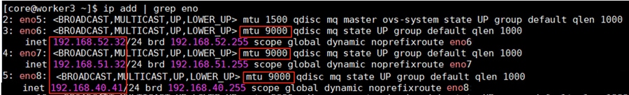
Ensure that each worker node is able to reach the target object storage IP address configured on the FlashBlade//S200 with lager transfer unit and without fragmenting the packet.
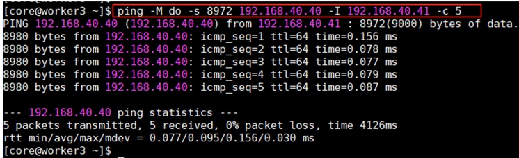
Install and Configure Portworx Enterprise on OpenShift with Pure Storage FlashArray
This chapter contains the following:
● Configure Physical Environment
● Portworx Enterprise Console Plugin for OpenShift
Portworx by Pure Storage is fully integrated with Red Hat OpenShift. Hence you can install and manage Portworx Enterprise from OpenShift web console itself. Portworx Enterprise can be installed with Pure Storage FlashArray as a cloud storage provider. This allows you to store your data on-premises with Pure Storage FlashArray while benefiting from Portworx Enterprise cloud drive features, such as:
● Automatically provisioning block volumes
● Expanding a cluster by adding new drives or expanding existing ones
● Support for PX-Backup and Autopilot
Portworx Enterprise will create and manage the underlying storage pool volumes on the registered arrays.
Note: Pure Storage recommends installing Portworx Enterprise with Pure Storage FlashArray Cloud Drives before using Pure Storage FlashArray Direct Access volumes.
This section provides the steps for installing Portworx Enterprise on OpenShift Container Platform running on Cisco UCSX-210C M7 bare metal servers. In this solution, Pure Storage FlashArray//XL170 is used as a backend storage connected over Ethernet to provide required Cloud Drives to be used by Portworx Enterprise. Figure 19 shows the high-level logical storage architecture of Portworx Enterprise deployment on Pure Storage FlashArray.
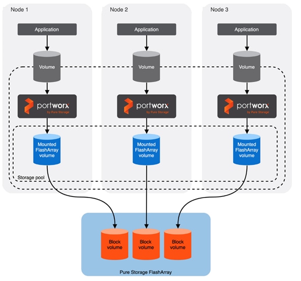
This is the high-level summary of the Portworx Enterprise implementation of distributed storage on a typical Kubernetes based Cluster:
● Portworx Enterprise runs on each worker node as Daemonset pod and based on the configuration information provided in the StorageClass spec, Portworx Enterprise provisions one or more volumes on Pure Storage FlashArray for each worker node.
● All these Pure Storage FlashArray volumes are pooled together to form one or more Distributed Storage Pools.
● When a user creates a PVC, Portworx Enterprise provisions the volume from the storage pool.
● The PVCs consume space on the storage pool, and if space begins to run low, Portworx Enterprise can add or expand drive space from Pure Storage FlashArray.
● If a worker node goes down for less than 2 minutes, Portworx Enterprise will reattach Pure Storage FlashArray volumes when it recovers. If a node goes down for more than two minutes, a storageless node in the same zone or fault domain will take up the volumes and assume the identity of the downed storage node.
These prerequisites must be met before installing the Portworx Enterprise on OpenShift with Pure Storage FlashArray:
● SecureBoot mode option must be disabled.
● The Pure Storage FlashArray should be time-synced with the same time service as the Kubernetes cluster.
● Pure Storage FlashArray must be running a minimum Purity//FA version of at least 4.8. Refer to the Supported models and versions topic for more information.
● Both multipath and iSCSI, if being used, should have their services enabled in systemd so that they start after reboots. These services are already enabled in systemd within the Red Hat CoreOS Linux.
Configure Physical Environment
Before you install Portworx Enterprise, ensure that your physical network is configured appropriately and that you meet the prerequisites. You must provide Portworx Enterprise with your Pure Storage FlashArray configuration details during installation:
● Each Pure Storage FlashArray management IP address can be accessed by each node.
● Your cluster contains an up-and-running Pure Storage FlashArray with an existing data plane connectivity layout (iSCSI, Fibre Channel).
● If you're using iSCSI, the storage node iSCSI initiators are on the same VLAN as the Pure Storage FlashArray iSCSI target ports.
● You have an API token for a user on your Pure Storage FlashArray with at least storage_admin permissions.
Procedure 1. Prepare for the Portworx Enterprise Deployment
Step 1. Secure the boot option already disabled at the Intersight Boot Policy level. To reconfirm at the OS level, SSH into any of the worker node from the installer VM and ensure that SecureBoot mode is disabled at the OS level.
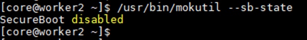
Step 2. Apply the following MachineConfig to the cluster configures each worker node with the following:
● Enable and start the multipathd.service with the specified multipath.conf configuration file.
● Enable and start the iscsid.service service.
● Applies the Queue Settings with Udev rules.
The settings of multipath and Udev rules are defined as shown below:
cat multipath.conf
blacklist {
devnode "^pxd[0-9]*"
devnode "^pxd*"
device {
vendor "VMware"
product "Virtual disk"
}
}
defaults {
user_friendly_names no
find_multipaths yes
polling_interval 10
}
devices {
device {
vendor "PURE"
product "FlashArray"
path_selector "service-time 0"
hardware_handler "1 alua"
path_grouping_policy group_by_prio
prio alua
failback immediate
path_checker tur
fast_io_fail_tmo 10
user_friendly_names no
no_path_retry 0
features 0
dev_loss_tmo 600
}
}
cat udevrules.txt
# Recommended settings for Pure Storage FlashArray.
# Use none scheduler for high-performance solid-state storage for SCSI devices
ACTION=="add|change", KERNEL=="sd*[!0-9]", SUBSYSTEM=="block", ENV{ID_VENDOR}=="PURE", ATTR{queue/scheduler}="none"
ACTION=="add|change", KERNEL=="dm-[0-9]*", SUBSYSTEM=="block", ENV{DM_NAME}=="3624a937*", ATTR{queue/scheduler}="none"
# Reduce CPU overhead due to entropy collection
ACTION=="add|change", KERNEL=="sd*[!0-9]", SUBSYSTEM=="block", ENV{ID_VENDOR}=="PURE", ATTR{queue/add_random}="0"
ACTION=="add|change", KERNEL=="dm-[0-9]*", SUBSYSTEM=="block", ENV{DM_NAME}=="3624a937*", ATTR{queue/add_random}="0"
# Spread CPU load by redirecting completions to originating CPU
ACTION=="add|change", KERNEL=="sd*[!0-9]", SUBSYSTEM=="block", ENV{ID_VENDOR}=="PURE", ATTR{queue/rq_affinity}="2"
ACTION=="add|change", KERNEL=="dm-[0-9]*", SUBSYSTEM=="block", ENV{DM_NAME}=="3624a937*", ATTR{queue/rq_affinity}="2"
# Set the HBA timeout to 60 seconds
ACTION=="add|change", KERNEL=="sd*[!0-9]", SUBSYSTEM=="block", ENV{ID_VENDOR}=="PURE", ATTR{device/timeout}="60"
The following is the MachineConfig file that takes the base64 encode results of the previous two files and copies them to the corresponding directory on each worker node. It also enables and starts iscsid and multipathd services:
cat multipathmcp.yaml
apiVersion: machineconfiguration.openshift.io/v1
kind: MachineConfig
metadata:
creationTimestamp:
labels:
machineconfiguration.openshift.io/role: worker
name: 99-worker-multipath-setting
spec:
config:
ignition:
version: 3.2.0
storage:
files:
- contents:
source: data:text/plain;charset=utf-8;base64,YmxhY2tsaXN0IHsKICAgICAgZGV2bm9kZSAiXnB4ZFswLTldKiIKICAgICAgZGV2bm9kZSAiXnB4ZCoiCiAgICAgIGRldmljZSB7CiAgICAgICAgdmVuZG9yICJWTXdhcmUiCiAgICAgICAgcHJvZHVjdCAiVmlydHVhbCBkaXNrIgogICAgICB9Cn0KZGVmYXVsdHMgewogdXNlcl9mcmllbmRseV9uYW1lcyBubwogZmluZF9tdWx0aXBhdGhzIHllcwogcG9sbGluZ19pbnRlcnZhbCAgMTAKfQpkZXZpY2VzIHsKICAgIGRldmljZSB7CiAgICAgICAgdmVuZG9yICAgICAgICAgICAgICAgICAgICJQVVJFIgogICAgICAgIHByb2R1Y3QgICAgICAgICAgICAgICAgICAiRmxhc2hBcnJheSIKICAgICAgICBwYXRoX3NlbGVjdG9yICAgICAgICAgICAgInNlcnZpY2UtdGltZSAwIgogICAgICAgIGhhcmR3YXJlX2hhbmRsZXIgICAgICAgICAiMSBhbHVhIgogICAgICAgIHBhdGhfZ3JvdXBpbmdfcG9saWN5ICAgICBncm91cF9ieV9wcmlvCiAgICAgICAgcHJpbyAgICAgICAgICAgICAgICAgICAgIGFsdWEKICAgICAgICBmYWlsYmFjayAgICAgICAgICAgICAgICAgaW1tZWRpYXRlCiAgICAgICAgcGF0aF9jaGVja2VyICAgICAgICAgICAgIHR1cgogICAgICAgIGZhc3RfaW9fZmFpbF90bW8gICAgICAgICAxMAogICAgICAgIHVzZXJfZnJpZW5kbHlfbmFtZXMgICAgICBubwogICAgICAgIG5vX3BhdGhfcmV0cnkgICAgICAgICAgICAwCiAgICAgICAgZmVhdHVyZXMgICAgICAgICAgICAgICAgIDAKICAgICAgICBkZXZfbG9zc190bW8gICAgICAgICAgICAgNjAwCiAgICB9Cn0K
filesystem: root
mode: 0644
overwrite: true
path: /etc/multipath.conf
- contents:
source: data:text/plain;charset=utf-8;base64,IyBSZWNvbW1lbmRlZCBzZXR0aW5ncyBmb3IgUHVyZSBTdG9yYWdlIEZsYXNoQXJyYXkuCiMgVXNlIG5vbmUgc2NoZWR1bGVyIGZvciBoaWdoLXBlcmZvcm1hbmNlIHNvbGlkLXN0YXRlIHN0b3JhZ2UgZm9yIFNDU0kgZGV2aWNlcwpBQ1RJT049PSJhZGR8Y2hhbmdlIiwgS0VSTkVMPT0ic2QqWyEwLTldIiwgU1VCU1lTVEVNPT0iYmxvY2siLCBFTlZ7SURfVkVORE9SfT09IlBVUkUiLCBBVFRSe3F1ZXVlL3NjaGVkdWxlcn09Im5vbmUiCkFDVElPTj09ImFkZHxjaGFuZ2UiLCBLRVJORUw9PSJkbS1bMC05XSoiLCBTVUJTWVNURU09PSJibG9jayIsIEVOVntETV9OQU1FfT09IjM2MjRhOTM3KiIsIEFUVFJ7cXVldWUvc2NoZWR1bGVyfT0ibm9uZSIKCiMgUmVkdWNlIENQVSBvdmVyaGVhZCBkdWUgdG8gZW50cm9weSBjb2xsZWN0aW9uCkFDVElPTj09ImFkZHxjaGFuZ2UiLCBLRVJORUw9PSJzZCpbITAtOV0iLCBTVUJTWVNURU09PSJibG9jayIsIEVOVntJRF9WRU5ET1J9PT0iUFVSRSIsIEFUVFJ7cXVldWUvYWRkX3JhbmRvbX09IjAiCkFDVElPTj09ImFkZHxjaGFuZ2UiLCBLRVJORUw9PSJkbS1bMC05XSoiLCBTVUJTWVNURU09PSJibG9jayIsIEVOVntETV9OQU1FfT09IjM2MjRhOTM3KiIsIEFUVFJ7cXVldWUvYWRkX3JhbmRvbX09IjAiCgojIFNwcmVhZCBDUFUgbG9hZCBieSByZWRpcmVjdGluZyBjb21wbGV0aW9ucyB0byBvcmlnaW5hdGluZyBDUFUKQUNUSU9OPT0iYWRkfGNoYW5nZSIsIEtFUk5FTD09InNkKlshMC05XSIsIFNVQlNZU1RFTT09ImJsb2NrIiwgRU5We0lEX1ZFTkRPUn09PSJQVVJFIiwgQVRUUntxdWV1ZS9ycV9hZmZpbml0eX09IjIiCkFDVElPTj09ImFkZHxjaGFuZ2UiLCBLRVJORUw9PSJkbS1bMC05XSoiLCBTVUJTWVNURU09PSJibG9jayIsIEVOVntETV9OQU1FfT09IjM2MjRhOTM3KiIsIEFUVFJ7cXVldWUvcnFfYWZmaW5pdHl9PSIyIgoKIyBTZXQgdGhlIEhCQSB0aW1lb3V0IHRvIDYwIHNlY29uZHMKQUNUSU9OPT0iYWRkfGNoYW5nZSIsIEtFUk5FTD09InNkKlshMC05XSIsIFNVQlNZU1RFTT09ImJsb2NrIiwgRU5We0lEX1ZFTkRPUn09PSJQVVJFIiwgQVRUUntkZXZpY2UvdGltZW91dH09IjYwIgo=
filesystem: root
mode: 0644
overwrite: true
path: /etc/udev/rules.d/99-pure-storage.rules
systemd:
units:
- enabled: true
name: iscsid.service
- enabled: true
name: multipathd.service
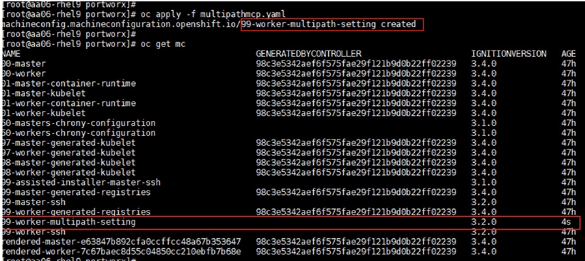
Step 3. This machine config is applied to each worker node one by one. To view the status of this process, from the cluster console go to Administration > Cluster Settings.
Step 4. After the MachineConfig is applied on all the worker nodes, ssh into one of the worker nodes and verify:
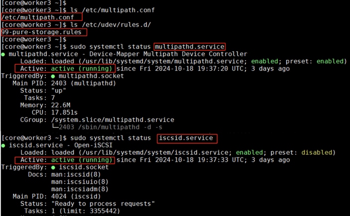
Step 5. From each worker node, ensure the Pure Storage FlashArray storage IPs are reachable with large packet size (8972) and without fragmenting the packets:
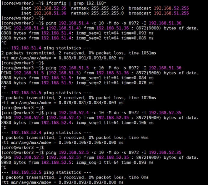
Step 6. Create Kubernetes secret object constituting the Pure Storage FlashArray API endpoints and API Tokens that Portworx Enterprise needs to communicate with and manage the Pure Storage FlashArray storage device.
Step 7. Log into Pure Storage FlashArray and go to Settings > Users and Polices. Create a dedicated user (for instance ocp-user) with storage Admin role for Portworx Enterprise authentication.
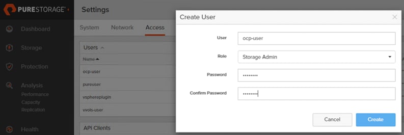
Step 8. Click the ellipses of the user previously created and select Create API Token. In the Create API Token wizard, set the number of weeks (for instance 24) for the API key to expire and click Create. A new API Token for the ocp-user will be created and will display. Copy the API key and preserve it since it will be used later to create Kubernetes Secret.
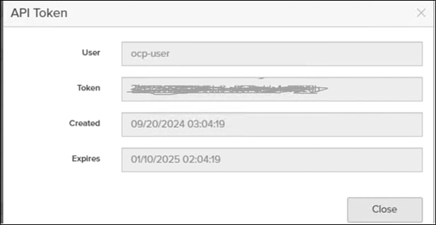
Step 9. Create Kubernetes secret with the API key (located above) using the following manifest:
## Create a json file constituting FlashArray Management IP addresses and API key created in the above step.
cat pure.json
{
"FlashArrays": [
{
"MgmtEndPoint": "10.103.0.55",
"APIToken": "< your API KEY >"
}
]
}
## secret name must match with below name
kubectl create secret generic px-pure-secret --namespace px --from-file=pure.json
Note: If multiple arrays configured with Availability Zones labels (AZs) are available, then you can use these AZ topology labels and enter those into pure.json to distinguish the arrays. For more details, go to: https://docs.portworx.com/portworx-enterprise/operations/operate-kubernetes/cluster-topology/csi-topology
Procedure 2. Deploy Portworx Enterprise
Step 1. Log into the OpenShift cluster console using the kubeadmin account and go to Operators > OperatorHub.
Step 2. In the right pane, enter Portworx Enterprise to filter the available operators in the Operator Hub. Select Portworx Enterprise and click Install.
Step 3. In the Operator Installation window, from the Installed Namespace drop-down list, select Create Project and create a new project (for instance px) and select the newly created project to install the Portworx Operator.
Step 4. Install the Portworx plugin for OpenShift by clicking Enable under the Console Plugin. Click Install.
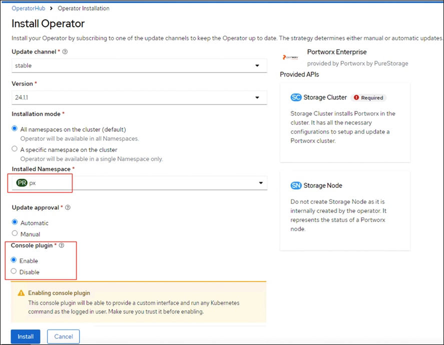
Note: The Portworx Console Plugin for OpenShift will be activated and shown only after installing the StorageCluster. Follow the below steps to create Portworx StorageCluster.
Step 5. When the Portworx operator is successfully installed, the StorageCluster needs to be created. To create the StorageCluster Specifications (manifest file) log into https://central.portworx.com/ and use your credentials and click Get Started.
Step 6. Select Portworx Enterprise and click Continue.
Step 7. From the Generate Spec page, select the latest Portworx version (version 3.1 was the latest when this solution was validated). Select Pure Storage FlashArray as the platform. Select OpenShift 4+ for the Distribution drop-down list, provide px for the Namespace field. Click Customize.
Step 8. Get the Kubernetes version by running kubectl version | grep -i 'Server Version'. Click Next.
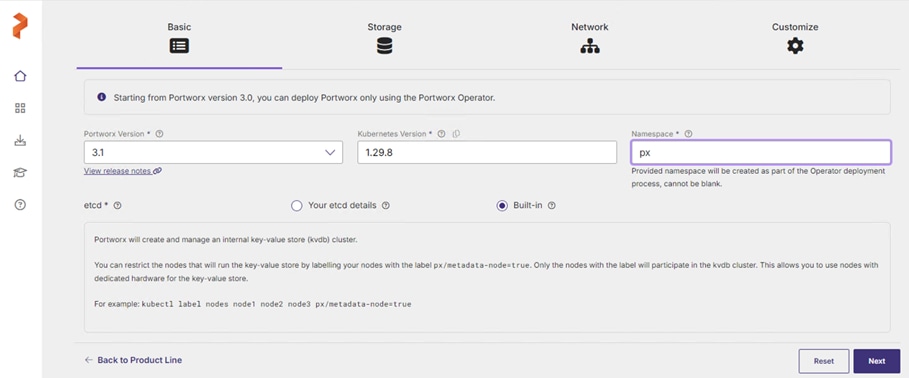
Step 9. From the Storage tab, select iSCSI for Storage Area Network. Provide the size of the Cloud drive and click plus (+) to add additional disks. Click Next.
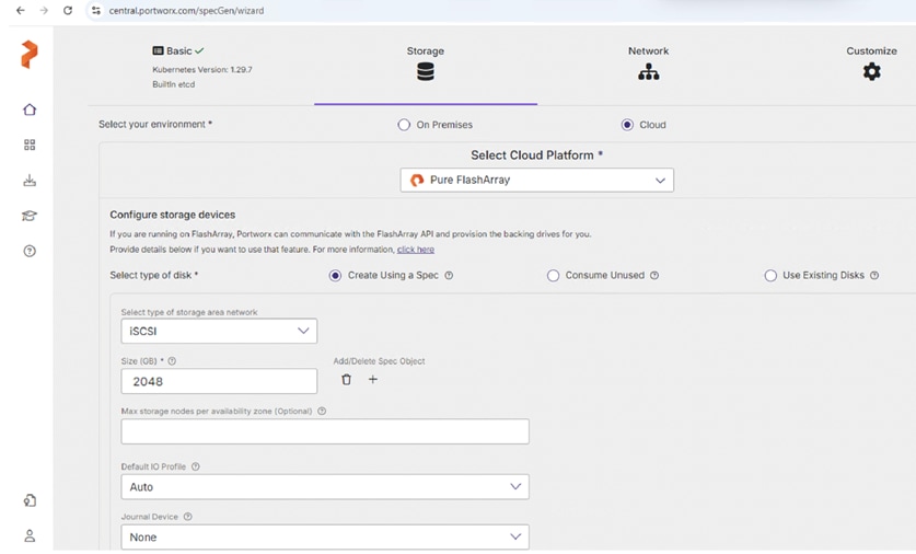
Step 10. From the Network tab, set Auto for both Data and Management Network Interfaces. Click Next.
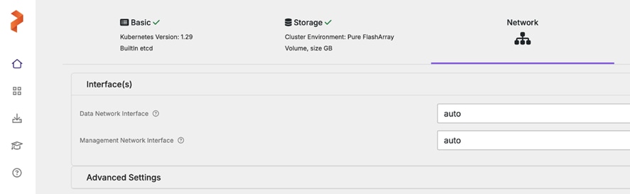
Step 11. From the Customize tab, click Auto for both Data and Management Network Interfaces. Click Next.
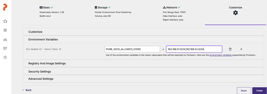
Note: Ensure to enter both the iSCSI network subnets. This enables the iSCSI volumes on the workers nodes to leverage all the available data paths to access target volumes.
Step 12. Click Advanced Settings, enter the name of the portworx cluster (for instance, ocp-pxclus). Click Finish. Click Download.yaml to download the StorageCluster specification file.
Step 13. From the OpenShift console, go to Operators > Installed Operators > Portworx Enterprise. Click the StorageCluster tab and click Create Storage Cluster to create StorageCluster. This opens the YAML view of Storage Cluster.
Step 14. Copy the contents of the spec file previously downloaded and paste it in the yaml body. Verify that both the iSCSI subnet networks are listed under env: as shown below. Click Create to create the StorageCluster.
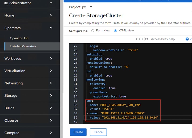
Step 15. Wait until all Portworx related pods are online.
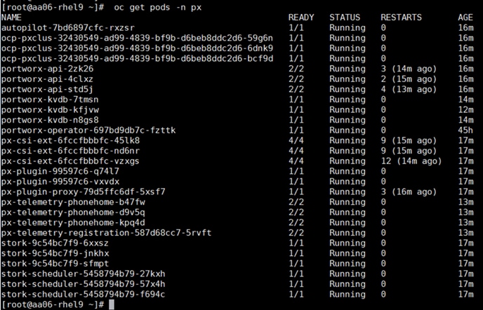
Step 16. Verify the cluster status by running the command on any worker node: sudo /opt/pwx/bin/pxctl status.
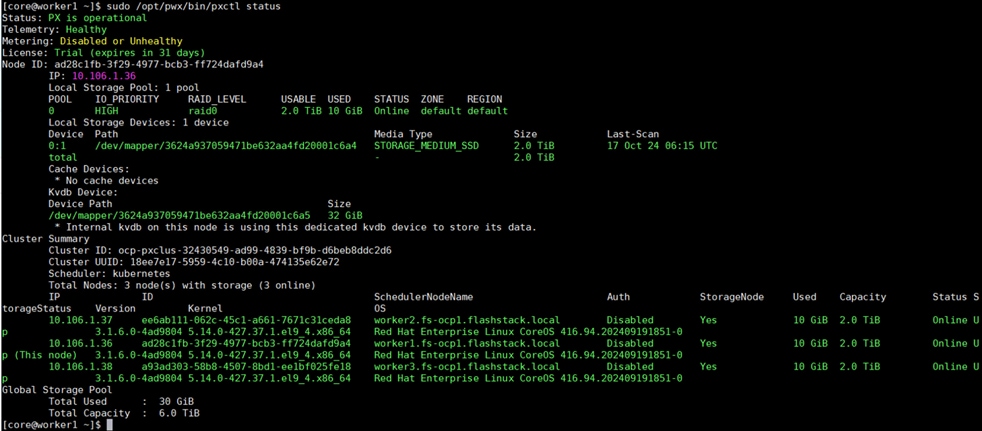
Step 17. Run the sudo multipath -ll command on one of the worker nodes to verify all four paths from the worker node to storage target are being used. As shown below, there are four active running paths for each volume:
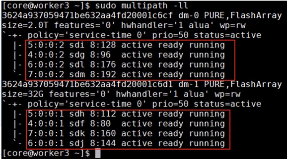
Now the Portworx StorageCluster is ready to use.
Procedure 3. Dynamic Volume Provisioning and Data Protection
Portworx by Pure Storage allows platform administrators to create custom Kubernetes StorageClasses to offer different classes of service to their developers. Administrators can customize things like the replication factors, snapshot schedules, file system types, io-profiles, etc. in their storage class definitions.
This procedure details how to create customized Storage Classes (SCs) for dynamic provisioning of volumes (PVs) using PersistentVolumeClaims (PVCs).
For instance, the following manifest file shows a sample file Storage Class for provisioning shared volume with ReadWriteMany (RWX) attribute to share the volume among multiple pods at the same time for read-write access. For provisioning volumes for typical application pods, predefined SCs can be leveraged.
## This SC is used to provision sharedv4 Service volumes (exposed as CLusterIP service) with two replicas.
## cat sharedv4-sc-svc.yaml
apiVersion: storage.k8s.io/v1
kind: StorageClass
metadata:
name: px-sharedv4-svc
provisioner: pxd.portworx.com
parameters:
repl: "2"
sharedv4: "true"
sharedv4_svc_type: "ClusterIP"
reclaimPolicy: Retain
allowVolumeExpansion: trueDeploy sample WordPress Application with Portworx Sharedv4 Service volumes
Step 1. Use the following manifests to create a sharedv4 service volumes to be consumed by multiple WordPress application accessing the sharev4 service volume (consumed by multiple WordPress pods) and ReadWriteOnce volume (Consumed by one MySQL pod):
## Deploying MySql database manifests
## create password.txt and update it with mysql root password.
kubectl create secret generic mysql-pass --from-file=./password.txt
## mysql PVC: cat mysql-pvc.yaml
apiVersion: v1
kind: PersistentVolumeClaim
metadata:
name: mysql-wordpress-pvc-rwo
annotations:
spec:
storageClassName: px-csi-db
accessModes:
- ReadWriteOnce
resources:
requests:
storage: 4Gi
## mysql deployment manifest: cat mysql-dep.yaml
apiVersion: apps/v1
kind: Deployment
metadata:
name: wordpress-mysql
labels:
app: wordpress
spec:
selector:
matchLabels:
app: wordpress
strategy:
type: Recreate
template:
metadata:
labels:
app: wordpress
tier: mysql
spec:
# Use the Stork scheduler to enable more efficient placement of the pods
schedulerName: stork
containers:
- image: mysql:5.6
imagePullPolicy:
name: mysql
env:
# $ kubectl create secret generic mysql-pass --from-file=password.txt
# make sure password.txt does not have a trailing newline
- name: MYSQL_ROOT_PASSWORD
valueFrom:
secretKeyRef:
name: mysql-pass
key: password.txt
ports:
- containerPort: 3306
name: mysql
volumeMounts:
- name: mysql-persistent-storage
mountPath: /var/lib/mysql
volumes:
- name: mysql-persistent-storage
persistentVolumeClaim:
claimName: mysql-wordpress-pvc-rwo
##worpess PVC created with ReadWriteMany access mode: cat wp-pvc.yaml
apiVersion: v1
kind: PersistentVolumeClaim
metadata:
name: wordpress-pvc-rwx
labels:
app: wordpress
spec:
storageClassName: px-sharedv4-rwx
accessModes:
- ReadWriteMany
resources:
requests:
storage: 7Gi
## Deployment manifest for wordpress application: cat wp-dep.yaml
apiVersion: apps/v1
kind: Deployment
metadata:
name: wordpress
labels:
app: wordpress
spec:
selector:
matchLabels:
app: wordpress
replicas: 3
strategy:
type: Recreate
template:
metadata:
labels:
app: wordpress
tier: frontend
spec:
# Use the Stork scheduler to enable more efficient placement of the pods
schedulerName: stork
containers:
- image: wordpress:4.8-apache
name: wordpress
imagePullPolicy:
env:
- name: WORDPRESS_DB_HOST
value: wordpress-mysql
- name: WORDPRESS_DB_PASSWORD
valueFrom:
secretKeyRef:
name: mysql-pass
key: password.txt
ports:
- containerPort: 80
name: wordpress
volumeMounts:
- name: wordpress-persistent-storage
mountPath: /var/www/html
volumes:
- name: wordpress-persistent-storage
persistentVolumeClaim:
claimName: wordpress-pvc-rwx
The following screenshot shows that 3 WordPress pods are created accessing the same sharedv4 volume with ReadWriteMany access mode and one mysql pod created with single volume with ReadWriteOnce access mode:
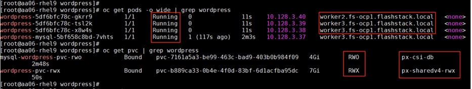
Sharedv4 Volume with ReadWriteMany (RWX) Access: Three WordPress pods are accessing the same sharedv4 volume with the ReadWriteMany access mode, meaning multiple pods can concurrently read from and write to this single volume. This is especially useful for applications like WordPress that may need to scale out to handle load but still rely on a shared data volume.
ReadWriteOnce (RWO) Access for MySQL: There is also a single MySQL pod accessing a volume with the ReadWriteOnce access mode, which allows only one pod to mount the volume at a time. This setup is common for databases, where concurrent access could lead to data inconsistencies.
This setup highlights Portworx's ability to support various access modes for different use cases, allowing flexible storage configurations that suit both shared applications (like WordPress) and single-instance databases (like MySQL). By providing the ReadWriteMany access mode with sharedv4, Portworx enables efficient scaling and resource usage, allowing applications to use shared storage across multiple pods and hosts
Snapshots and Clones: Portworx Enterprise offers data protection of volumes using volume snapshots and restore them for point in time recovery of the data. Any Storage Class that implements portworx csi driver pxd.portworx.com supports volume Snapshots.
Step 2. Run the following scripts to create the VolumeSnapshotClass, a PVC and then a Snapshot of a PVC and then restore the snapshot as a new PVC.
## For Openshift platform, px-csi-account service account needs to be added to the privileged security context.
oc adm policy add-scc-to-user privileged system:serviceaccount:kube-system:px-csi-account
## Now creat VolumeSnapshotClass using below manifest
## cat VolumeStroageClass.yaml
apiVersion: snapshot.storage.k8s.io/v1
kind: VolumeSnapshotClass
metadata:
name: px-csi-snapclass
annotations:
snapshot.storage.kubernetes.io/is-default-class: "true"
driver: pxd.portworx.com
deletionPolicy: Delete
parameters:
csi.openstorage.org/snapshot-type: local
Step 3. Use the following sample manifest to create a sample PVC:
## cat px-snaptest-pvc.yaml
kind: PersistentVolumeClaim
apiVersion: v1
metadata:
name: px-snaptest-pvc
spec:
storageClassName: px-csi-db. ## Any Storage Class can be used which implements Portworx CSI driver.
accessModes:
- ReadWriteOnce
resources:
requests:
storage: 2Gi
## Assume this pvc is attached to a pod and the pod has written some data into the pvc.
## Now create Snapshot of the above volume. It can be created using UI also.
## cat create-snapshot-snaptest-pvc.yaml
apiVersion: snapshot.storage.k8s.io/v1
kind: VolumeSnapshot
metadata:
name: px-snaptest-pvc-snap1
spec:
volumeSnapshotClassName: px-csi-snapclass
source:
persistentVolumeClaimName: px-snaptest-pvc. ## the name of the pvc
The following screenshot shows px-snaptest-pvc-snap1 is the snapshot of the PVC px-snaptest-pvc:
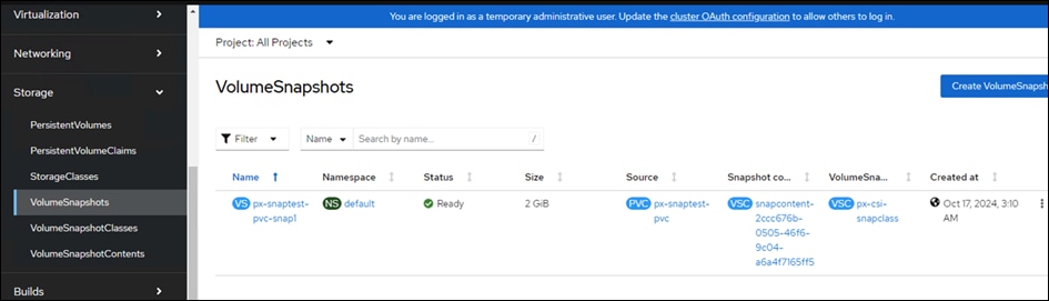
Step 4. You can now restore this as snapshot as a new PVC and then can be mounted to any other pod.
Step 5. Click the ellipses of the snapshot and select Restore as new PVC. In the Restore as new PVC window, click Restore.
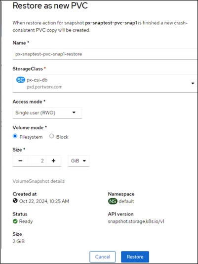
Step 6. You can view the original and restored PVC under PVC list.
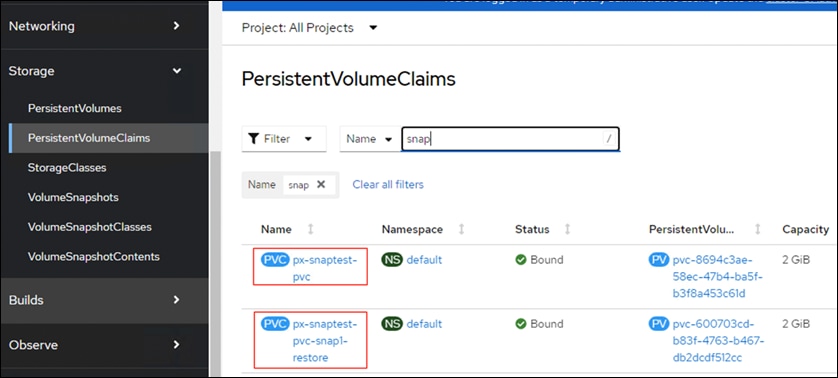
Step 7. To clone of a PVC (px-snaptest-pvc), click three of the PVC and select Clone PVC. Click Clone.
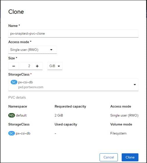
Portworx Enterprise Console Plugin for OpenShift
Portworx by Pure Storage has built an OpenShift Dynamic console plugin that enables single-pane-of-glass management of storage resources running on Red Hat OpenShift clusters. This allows platform administrators to use the OpenShift web console to manage not just their applications and their OpenShift cluster, but also their Portworx Enterprise installation and their stateful applications running on OpenShift.
This plugin can be installed with a single click during the Installation of Portworx Operator as explained in the previous sections. Once the plugin is enabled, the Portworx Operator will automatically install the plugin pods in the same OpenShift project as the Portworx storage cluster. When the pods are up and running, administrators will see a message in the OpenShift web console to refresh their browser window for the Portworx tabs to show up in the UI.
With this plugin, Portworx has built three different UI pages, including a Portworx Cluster Dashboard that shows up in the left navigation menu, a Portworx tab under Storage > Storage Class section, and another Portworx tab under Storage > Persistent Volume Claims.
Portworx Cluster Dashboard
Platform administrators can use the Portworx Cluster Dashboard to monitor the status of their Portworx Storage Cluster and their persistent volumes and storage nodes. Here are a few operations that are now streamlined by the OpenShift Dynamic plugin from Portworx.
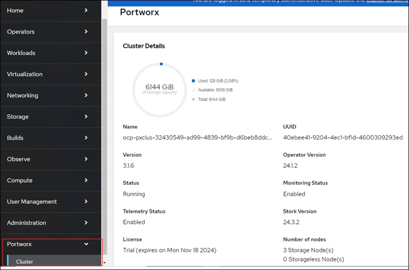
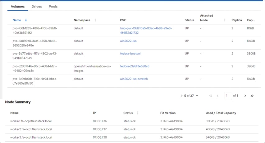
To obtain detailed inventory information of the Portworx Cluster, click the Drives and Pools tabs.
Portworx PVC Dashboard
This dashboard shows some of the important attributes of a PVC like Replication Factor, node details of replicas, attached node and so on. You may have to use multiple pxctl inspect volume CLI commands to get these details. Instead, all this information can be found in Console Plugin.
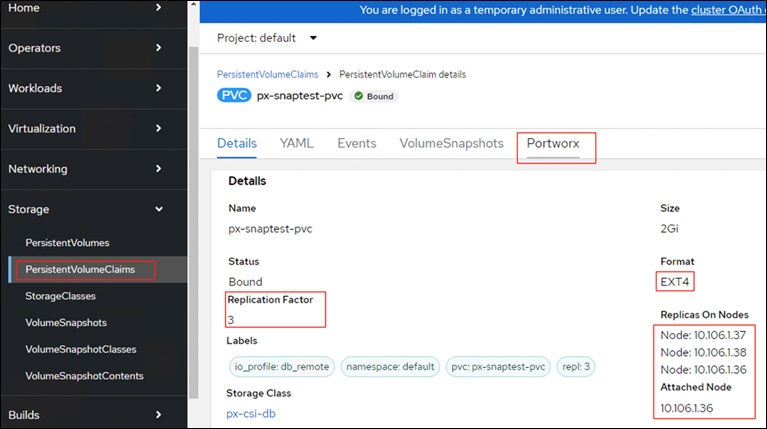
Portworx StorageClass Dashboard
From the Portworx storage cluster tab, administrators can get details about the custom parameters set for each storage class, the number of persistent volumes dynamically provisioned using the storage class, and a table that lists all the persistent volumes deployed using that storage class. The OpenShift dynamic plugin eliminates the need for administrators to use multiple “kubectl get” and “kubectl describe” commands to find all these details—instead, they can just use a simple UI to monitor their storage classes.
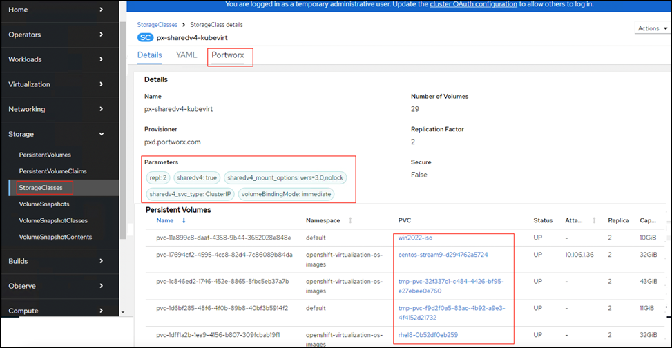
RAG Pipeline Installation and Configuration
This chapter contains the following:
● NVIDIA NIM Operator and NIMs
● Access Services and Application
The reference RAG Blueprint leverages the NIMs deployed for LLMs, Text Embedding, and Text Reranking. It uses the Milvus vector database to store the vector embeddings.
Note: It is required to deploy NIMs, and the Milvus Vector database first and then deploy RAG Blueprint.
NIMs can be installed independently using its respective helm charts from https://catalog.ngc.nvidia.com/helm-charts. It can also be installed and managed using NVIDIA NIM Operator. In this design, NIMs will be installed and managed using NVIDIA NIM Operator.
Procedure 1. Install NIM Operator
Step 1. In the Red Hat OpenShift console, go to Operators > OperatorHub.
Step 2. Search for NVIDIA NIM Operator.
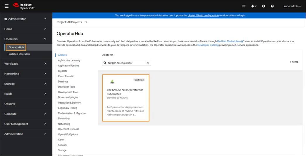
Step 3. Click Install.
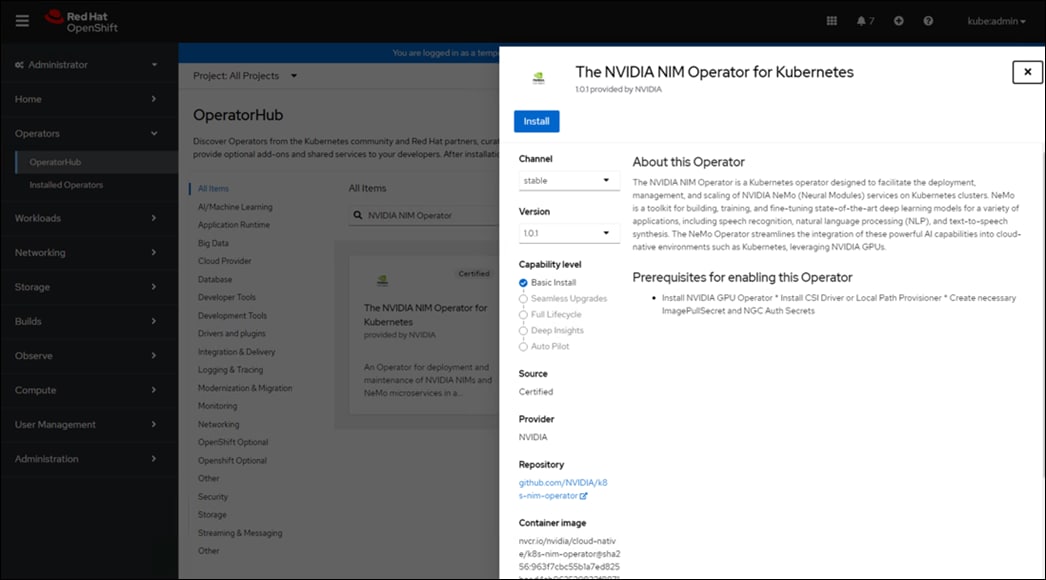
Step 4. Retain Installed Namespace as openshift-operators. Click Install.
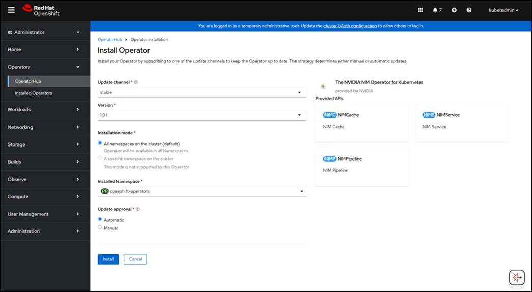
Create Caching Models
NIM Operator uses a custom resource called NIM cache (nimcaches.apps.nvidia.com). This custom resource enables downloading models from NVIDIA NGC and persisting them on Portworx persistent storage.
One advantage to caching a model is that when multiple instances of the same NIM microservice start, the microservices use the single cached model. However, caching is optional. Without caching, each NIM microservice instance downloads a copy of the model when it starts.
It is recommended to cache the models for NVIDIA NIM microservices. By caching a model, the microservice startup time is improved. For deployments that scale to more than one NIM microservice pod, a single cached model in persistent volume with a storage class from Portworx provisioner can serve multiple pods.
This section provides the procedures to create caching models for LLMs, Text Embedding, and Text Reranking.
Procedure 1. Create namespace
Step 1. To create the namespace, run the following command:
oc create namespace nim
Procedure 2. Secrets for NGC API key
Step 1. NIM cache uses the NGC API key as an image pull secret to download container images and models from NVIDIA NGC. Add a Docker registry secret for downloading the NIM container image from NVIDIA NGC:
oc create secret -n nim docker-registry ngc-secret \
--docker-server=nvcr.io \
--docker-username='$oauthtoken' \
--docker-password=<ngc-api-key>
Step 2. Add a generic secret that the model puller init container uses to download the model from NVIDIA NGC:
oc create secret -n nim generic ngc-api-secret \
--from-literal=NGC_API_KEY=<ngc-api-key>
NIM cache for LLM
Refer to the following sample manifest as an example:
apiVersion: apps.nvidia.com/v1alpha1
kind: NIMCache
metadata:
name: meta-llama3-8b
spec:
source:
ngc:
modelPuller: nvcr.io/nim/meta/llama3-8b-instruct:1.0.3
pullSecret: ngc-secret
authSecret: ngc-api-secret
model:
gpus:
- product: "l40s"
engine: tensorrt_llm
tensorParallelism: "1"
storage:
pvc:
create: true
storageClass: <storage_class_naME>
size: "100Gi"
volumeAccessMode: ReadWriteMany
When you create a NIM cache resource, the NIM Operator starts a pod that lists the available model profiles. The Operator creates a config map of the model profiles.
If you specify one or more model profile IDs to cache, the Operator starts a job that caches the model profiles that you specified.
If you did not specify model profile IDs but do specify engine: tensorrt_llm or engine: tensorrt, the Operator attempts to match the model profiles with the GPUs on the nodes in the cluster. The Operator uses the value of the nvidia.com/gpu.product node label that is set by Node Feature Discovery.
You can let the Operator automatically detect the model profiles to cache or you can constrain the model profiles by specifying values for spec.source.ngc.model, such as the engine, GPU model, and so on, that must match the model profile.
More information about the option is available here: https://docs.nvidia.com/nim-operator/latest/cache.html
NIM Cache for Text Embedding
Refer to the following example sample manifest:
apiVersion: apps.nvidia.com/v1alpha1
kind: NIMCache
metadata:
name: llama-3.2-nv-embedqa-1b-v2
spec:
source:
ngc:
modelPuller: nvcr.io/nim/nvidia/llama-3.2-nv-embedqa-1b-v2:latest
pullSecret: ngc-secret
authSecret: ngc-api-secret
model:
profiles:
- all
storage:
pvc:
create: true
storageClass: <storage_class_name>
size: "100Gi"
volumeAccessMode: ReadWriteMany
NIM Cache for Text Reranking
Refer to the following example sample manifest:
apiVersion: apps.nvidia.com/v1alpha1
apiVersion: apps.nvidia.com/v1alpha1
kind: NIMCache
metadata:
name: rerankqa
spec:
source:
ngc:
modelPuller: nvcr.io/nim/nvidia/llama-3.2-nv-rerankqa-1b-v2:latest
pullSecret: ngc-secret
authSecret: ngc-api-secret
model:
profiles:
- all
storage:
pvc:
create: true
storageClass: kubevirt
size: "100Gi"
volumeAccessMode: ReadWriteMany
Procedure 1. Create Resources
Step 1. Apply the YAML manifests to all three models:
oc apply -n nim -f <yaml_manifest_name>
Step 2. View the NIM cache resource to view the status:
[root@aa06-rhel9 blueprint]# oc get nimcaches.apps.nvidia.com -n nim
NAME STATUS PVC AGE
llama-3.2-nv-embedqa-1b-v2 Ready llama-3.2-nv-embedqa-1b-v2-pvc 11d
meta-llama3.1-8b Ready meta-llama3.1-8b-pvc 11d
rerankqa Ready rerankqa-pvc 11d
Create Services
NIM Services (nimservices.apps.nvidia.com) custom resource represents a NIM microservice. Adding and updating a NIM service resource creates a Kubernetes deployment for the microservice in a namespace. The custom resource supports using a model from an existing NIM cache resource or a persistent volume claim.
NIM Service for LLM
Refer to the following example sample manifest:
apiVersion: apps.nvidia.com/v1alpha1
kind: NIMService
metadata:
name: llm
spec:
image:
repository: nvcr.io/nim/meta/llama-3.1-8b-instruct
tag: 1.3.3
pullPolicy: IfNotPresent
pullSecrets:
- ngc-secret
authSecret: ngc-api-secret
storage:
nimCache:
name: meta-llama3.1-8b
profile: ''
replicas: 1
resources:
limits:
nvidia.com/gpu: 1
expose:
service:
type: NodePort
port: 8000
NIM Service for Text Embedding
Refer to the following example sample manifest:
apiVersion: apps.nvidia.com/v1alpha1
kind: NIMService
metadata:
name: embedqa
spec:
image:
repository: nvcr.io/nim/nvidia/llama-3.2-nv-embedqa-1b-v2
tag: latest
pullPolicy: IfNotPresent
pullSecrets:
- ngc-secret
authSecret: ngc-api-secret
storage:
nimCache:
name: llama-3.2-nv-embedqa-1b-v2
profile: ''
replicas: 1
resources:
limits:
nvidia.com/gpu: 1
expose:
service:
type: ClusterIP
port: 8000
NIM Service for Text Reranking
Refer to the following example sample manifest:
apiVersion: apps.nvidia.com/v1alpha1
kind: NIMService
metadata:
name: rerankqa
spec:
image:
repository: nvcr.io/nim/nvidia/llama-3.2-nv-rerankqa-1b-v2
tag: latest
pullPolicy: IfNotPresent
pullSecrets:
- ngc-secret
authSecret: ngc-api-secret
storage:
nimCache:
name: rerankqa
profile: ''
replicas: 1
resources:
limits:
nvidia.com/gpu: 1
expose:
service:
type: ClusterIP
port: 8000
View the NIM services custom resources:
oc get nimservices.apps.nvidia.com -n nim
Create NIM Pipelines
As an alternative to managing NIM services individually using multiple NIMService custom resources, you can manage multiple NIM services using one NIMPipeline custom resource.
The following sample manifest deploys all NIMs mentioned above without creating individual NIM services:
apiVersion: apps.nvidia.com/v1alpha1
kind: NIMPipeline
metadata:
name: pipeline-all
spec:
services:
- name: llm
enabled: true
spec:
image:
repository: nvcr.io/nim/meta/llama-3.1-8b-instruct
tag: 1.3.3
pullPolicy: IfNotPresent
pullSecrets:
- ngc-secret
authSecret: ngc-api-secret
storage:
nimCache:
name: meta-llama3.1-8b
profile: ''
replicas: 1
resources:
limits:
nvidia.com/gpu: 1
expose:
service:
type: ClusterIP
port: 8000
- name: embedqa
enabled: true
spec:
image:
repository: nvcr.io/nim/nvidia/llama-3.2-nv-embedqa-1b-v2
tag: latest
pullPolicy: IfNotPresent
pullSecrets:
- ngc-secret
authSecret: ngc-api-secret
storage:
nimCache:
name: llama-3.2-nv-embedqa-1b-v2
profile: ''
replicas: 1
resources:
limits:
nvidia.com/gpu: 1
expose:
service:
type: ClusterIP
port: 8000
- name: rerankqa
enabled: true
spec:
image:
repository: nvcr.io/nim/nvidia/llama-3.2-nv-rerankqa-1b-v2
tag: latest
pullPolicy: IfNotPresent
pullSecrets:
- ngc-secret
authSecret: ngc-api-secret
storage:
nimCache:
name: rerankqa
profile: ''
replicas: 1
resources:
limits:
nvidia.com/gpu: 1
expose:
service:
type: ClusterIP
port: 8000
More information about NIM Pipelines is available here: https://docs.nvidia.com/nim-operator/latest/pipelines.html
Procedure 1. Verification
After all the NIMs are deployed, you can verify the status of the services by calling “/v1/health/ready” API endpoint. First, get the services exposed to access the LLM, Embedding and Reranking models.
Step 1. Note that the service names will be the same as name given while creating the NIM Service. In the previous example, NIM service for Llama-3.1 is created using name llm, Llama-3.2 Text Embedding NIM with embedqa and Llama 3.2 1B Reranking with the name rerankqa:
[root@aa06-rhel9 blueprint]# oc get svc -n nim
NAME TYPE CLUSTER-IP EXTERNAL-IP PORT(S)
embedqa NodePort 172.30.103.111 <none> 8000:30765/TCP
llm NodePort 172.30.73.126 <none> 8000:30604/TCP
rerankqa NodePort 172.30.160.141 <none> 8000:32630/TCP
[root@aa06-rhel9 blueprint]# oc get svc -o custom-columns=NAME:.metadata.name,PORT_TYPE:.spec.type,NODE_PORT:.spec.ports[*].nodePort
NAME PORT_TYPE NODE_PORT
embedqa NodePort 30765
llm NodePort 30604
rerankqa NodePort 32630
Step 2. From the previous output, Llama-3.1 is available using NodePort 30604, embedding model at 30765 and rerank model at 32630. All services with ClusterIP Port 8000.
Step 3. Get the IP or DNS name of the node ports by running the following command:
[root@aa06-rhel9 blueprint]# oc get nodes -o wide
Step 4. Verify the status of each service running using “/v1/health/ready” endpoint:
[root@aa06-rhel9 blueprint]# curl http://10.106.1.33:30604/v1/health/ready
{"object":"health.response","message":"Service is ready."}
[root@aa06-rhel9 blueprint]# curl http://10.106.1.33:30765/v1/health/ready
{"object":"health-response","message":"Service is ready."}
[root@aa06-rhel9 blueprint]# curl http://10.106.1.33:32630/v1/health/ready
{"object":"health-response","message":"Service is ready."}
This section provides the procedures to deploy the Milvus vector database:
● Before deploying Milvus vector database deployment, ensure the following pre-requisites are configured on the FlashBlade//S.
● For the Object storage traffic between the FlashBlade//S and workers nodes, create required Link Aggregation Groups (LAGs), Subnets and Interface on the FlashBlade//S and assign IP address to the Interface.
● On each worker node, ensure an interface is configured with IP addresses in the same subnet as that of FlashBlade//S interface and ensure IPs are reachable from each other.
● In the FlashBlade//S array, ensure that an account with at least one User ID is created and configured with required access policy and Access key. Also ensure, at least one Bucket is created and mapped to the account created in the above step.
In this architecture, FlashBlade//S is used as S3 compatible backend object storage as required by Milvus vector database for storing Milvus collections (Vector embeddings) and Indexes. While the FlashArray//XL170 is used for storing other Milvus components like Pulsar’s bookie journal, Zookeeper and so on.
Procedure 1. Configure Portworx storage class
Step 1. Run the following script to configure one of portworx storage classes configured with FlashArray //XL170 and back-end storage as ‘Default storage class’:
kubectl patch storageclass <<your Preffered StorageClass Name>> -p '{"metadata": {"annotations":{"storageclass.kubernetes.io/is-default-class":"true"}}}'
Step 2. Ensure the routingViaHost is set to true by running the below script. This will ensure the Milvus Pod to directly access the FlashBlade//S interfaces via worker node network interfaces for object storage traffic:
oc patch Network.operator.openshift.io cluster --type=merge \
--patch '{
"spec":{
"defaultNetwork":{
"ovnKubernetesConfig":{
"gatewayConfig": {
"ipForwarding": "Global",
"routingViaHost": true
}}}}}'
oc describe Network.operator.openshift.io cluster
Name: cluster
Namespace:
Labels: <none>
Annotations: <none>
API Version: operator.openshift.io/v1
Kind: Network
Metadata:
Creation Timestamp: 2025-01-02T09:32:18Z
Generation: 157
Resource Version: 54848544
UID: a44accc1-8efa-4635-aa52-ca6defdf21af
Spec:
Cluster Network:
Cidr: 10.128.0.0/14
Host Prefix: 23
Default Network:
Ovn Kubernetes Config:
Egress IP Config:
Gateway Config:
Ip Forwarding: Global
ipv4:
ipv6:
Routing Via Host: true
Geneve Port: 6081
Ipsec Config:
---
---
Step 3. Run the following script on oc terminal to update the Security context (SCC) to allow anyuid for the service accounts created by the milvus helm chart:
oc adm policy add-scc-to-user anyuid -z milvus-deployment-pulsarv3-bookie -n milvus
oc adm policy add-scc-to-user anyuid -z milvus-deployment-pulsarv3-broker-acct -n milvus
oc adm policy add-scc-to-user anyuid -z milvus-deployment-pulsarv3-proxy -n milvus
oc adm policy add-scc-to-user anyuid -z milvus-deployment-pulsarv3-recovery -n milvus
oc adm policy add-scc-to-user anyuid -z milvus-deployment-pulsarv3-zookeeper -n milvus
oc adm policy add-scc-to-user anyuid -z default -n milvus
Before proceeding with the Milvus deployment, gather the following details listed in Table 21 and keep them available.
Table 21. Storage Details required for Vector Database deployment
| Item |
Details |
| Object Storage IP Interface IP |
192.168.40.40 |
| Port |
80 |
| Access Key |
<<The Access Key generated while configuring the user id in the FlashBlade//S>> |
| Secret Key |
<< The Secret Key generated while configuring the user id in the FlashBlade//S >> |
| Bucket Name |
aa06-milvus-bkt |
| Worker node IPs designated for Object storage traffic |
192.168.40.41, 192.168.40.42, 192.168.40.43 |
| Default Storage Class created by Portworx |
<< Name of your Default Portworx Storage Class>> |
Procedure 2. Milvus Deployment with Pure Storage FlashBlade//S
Step 1. Create a new namespace for milvus:
oc create namespace milvus
Step 2. Add the milvus repository:
helm repo add milvus https://zilliztech.github.io/milvus-helm/
Step 3. Update the helm repository:
helm repo update
Note: The RAG deployment can work with either Standalone or Distributed Milvus vector database. For more details on the type of Milvus vector database is suitable for your RAG deployment, refer: https://zilliz.com/blog/choose-the-right-milvus-deployment-mode-ai-applications
Step 4. Create a file named custom_value.yaml for customizing the Milvus deployment. Specify Attu details, milvus version that supports GPU based indexes, number of replicas, GPU resources and FlashBlade details for object storage as shown in sample manifest file:
###################custom_values.yaml for distributed Milvus deployment###########################
attu:
enabled: true
name: attu
image:
repository: zilliz/attu
tag: v2.3.10
pullPolicy: IfNotPresent
service:
annotations: {}
labels: {}
type: NodePort
port: 3000
# loadBalancerIP: ""
resources: {}
podLabels: {}
ingress:
enabled: false
ingressClassName: ""
annotations: {}
# Annotation example: set nginx ingress type
# kubernetes.io/ingress.class: nginx
labels: {}
hosts:
- milvus-attu.local
tls: []
# - secretName: chart-attu-tls
# hosts:
# - milvus-attu.local
## For this testing, Milvus vector database version 2.5.2 is used. Set the tag to “latest” if you would like to use latest version
## For HSNW CPU based index, use version v2.5.2; For GPU-Optmized Indexes of Milvus, use version v2.5.2-gpu
image:
all:
repository: milvusdb/milvus
tag: v2.5.2-gpu
pullPolicy: IfNotPresent
## For HSNW CPU based index, do not mentioned below section that contains the GPU details.
## Update the number of GPUs to be assigned to the Query and Index nodes
indexNode:
resources:
requests:
nvidia.com/gpu: "1"
limits:
nvidia.com/gpu: "1"
queryNode:
resources:
requests:
nvidia.com/gpu: "1"
limits:
nvidia.com/gpu: "1"
dataNode:
replicas: 2
minio:
enabled: false
# Update host, accessKey, secretKey and bucketName based on your setup
externalS3:
enabled: true
host: "192.168.40.40"
port: "80"
accessKey: "<<Access Key>>"
secretKey: "<<Secret Key>>"
useSSL: false
bucketName: "aa06-milvus-bkt"
rootPath: ""
useIAM: false
cloudProvider: ""
iamEndpoint:
#####################custom_values.yaml for standalone Milvus deployment #############
attu:
enabled: true
name: attu
image:
repository: zilliz/attu
tag: v2.3.10
pullPolicy: IfNotPresent
service:
annotations: {}
labels: {}
type: NodePort
port: 3000
# loadBalancerIP: ""
resources: {}
podLabels: {}
ingress:
enabled: false
ingressClassName: ""
annotations: {}
# Annotation example: set nginx ingress type
# kubernetes.io/ingress.class: nginx
labels: {}
hosts:
- milvus-attu.local
tls: []
# - secretName: chart-attu-tls
# hosts:
# - milvus-attu.local
## For this testing, Milvus vector database version 2.5.2 is used. Set the tag to “latest” if you would like to use latest version
## For HSNW CPU based index, use version v2.5.2; For GPU-Optmized Indexes of Milvus, use version v2.5.2-gpu
image:
all:
repository: milvusdb/milvus
tag: v2.5.2-gpu
pullPolicy: IfNotPresent
## For HSNW CPU based index, do not make use of GPUs. Hence GPU section can be ignored.
## Update the number of GPUs to be assigned to the Query and Index nodes
standalone:
resources:
requests:
nvidia.com/gpu: "1"
limits:
nvidia.com/gpu: "1"
minio:
enabled: false
# Update host, accessKey, secretKey and bucketName based on your setup
externalS3:
enabled: true
host: "192.168.40.40"
port: "80"
accessKey: "<<Access Key>>"
secretKey: "<<Secret Key>>"
useSSL: false
bucketName: "aa06-milvus-bkt"
rootPath: ""
useIAM: false
cloudProvider: ""
iamEndpoint:
Step 5. Install the helm chart and point to the previously created file using -f argument as shown below:
### use below command to deploy distributed Milvus vector database
helm install milvus-deployment milvus/milvus -f custom_value.yaml -n milvus
### use below command to deploy standard Milvus vector database
helm install milvus-deployment milvus/milvus --set cluster.enabled=false --set etcd.replicaCount=1 --set minio.mode=standalone --set pulsar.enabled=false -f s3-milvus-gpuimage_stand.yaml -n milvus
Step 6. Check the status of the pods:
oc get pods -n milvus
All pods should be running and in a ready state within couple of minutes:
[root@aa06-rhel9 milvus]# oc get all -n milvus
Warning: apps.openshift.io/v1 DeploymentConfig is deprecated in v4.14+, unavailable in v4.10000+
Warning: kubevirt.io/v1 VirtualMachineInstancePresets is now deprecated and will be removed in v2.
NAME READY STATUS RESTARTS AGE
pod/milvus-cli 1/1 Running 0 59d
pod/milvus-deployment-attu-c5f766b57-gnkrx 1/1 Running 0 4m55s
pod/milvus-deployment-datanode-6ffcfc775b-rd8sz 1/1 Running 2 (4m33s ago) 4m55s
pod/milvus-deployment-datanode-6ffcfc775b-s7mpb 1/1 Running 2 (4m33s ago) 4m55s
pod/milvus-deployment-etcd-0 1/1 Running 0 4m55s
pod/milvus-deployment-etcd-1 1/1 Running 0 4m55s
pod/milvus-deployment-etcd-2 1/1 Running 0 4m55s
pod/milvus-deployment-indexnode-85987bc575-fbxm4 1/1 Running 2 (4m33s ago) 4m55s
pod/milvus-deployment-mixcoord-76cc8fd974-ctq5p 1/1 Running 2 (4m33s ago) 4m55s
pod/milvus-deployment-proxy-6f88b49dd6-xqvk9 1/1 Running 2 (4m33s ago) 4m55s
pod/milvus-deployment-pulsarv3-bookie-0 1/1 Running 0 4m55s
pod/milvus-deployment-pulsarv3-bookie-1 1/1 Running 0 4m55s
pod/milvus-deployment-pulsarv3-bookie-2 1/1 Running 0 4m55s
pod/milvus-deployment-pulsarv3-bookie-init-szcb4 0/1 Completed 0 4m55s
pod/milvus-deployment-pulsarv3-broker-0 1/1 Running 0 4m55s
pod/milvus-deployment-pulsarv3-broker-1 1/1 Running 0 4m55s
pod/milvus-deployment-pulsarv3-proxy-0 1/1 Running 0 4m55s
pod/milvus-deployment-pulsarv3-proxy-1 1/1 Running 0 4m55s
pod/milvus-deployment-pulsarv3-pulsar-init-n7lnf 0/1 Completed 0 4m55s
pod/milvus-deployment-pulsarv3-recovery-0 1/1 Running 0 4m55s
pod/milvus-deployment-pulsarv3-zookeeper-0 1/1 Running 0 4m55s
pod/milvus-deployment-pulsarv3-zookeeper-1 1/1 Running 0 4m55s
pod/milvus-deployment-pulsarv3-zookeeper-2 1/1 Running 0 4m55s
pod/milvus-deployment-querynode-7d8f4b9f49-5pmkb 1/1 Running 2 (4m33s ago) 4m55s
NAME TYPE CLUSTER-IP EXTERNAL-IP PORT(S) AGE
service/milvus-deployment ClusterIP 172.30.199.87 <none> 19530/TCP,9091/TCP 4m55s
service/milvus-deployment-attu NodePort 172.30.203.187 <none> 3000:30245/TCP 4m55s
service/milvus-deployment-datanode ClusterIP None <none> 9091/TCP 4m55s
service/milvus-deployment-etcd ClusterIP 172.30.29.129 <none> 2379/TCP,2380/TCP 4m55s
service/milvus-deployment-etcd-headless ClusterIP None <none> 2379/TCP,2380/TCP 4m55s
service/milvus-deployment-indexnode ClusterIP None <none> 9091/TCP 4m55s
service/milvus-deployment-mixcoord ClusterIP 172.30.36.164 <none> 9091/TCP 4m55s
service/milvus-deployment-pulsarv3-bookie ClusterIP None <none> 3181/TCP,8000/TCP 4m55s
service/milvus-deployment-pulsarv3-broker ClusterIP None <none> 8080/TCP,6650/TCP 4m55s
service/milvus-deployment-pulsarv3-proxy ClusterIP 172.30.103.87 <none> 80/TCP,6650/TCP 4m55s
service/milvus-deployment-pulsarv3-recovery ClusterIP None <none> 8000/TCP 4m55s
service/milvus-deployment-pulsarv3-zookeeper ClusterIP None <none> 8000/TCP,2888/TCP,3888/TCP,2181/TCP 4m55s
service/milvus-deployment-querynode ClusterIP None <none> 9091/TCP 4m55s
NAME READY UP-TO-DATE AVAILABLE AGE
deployment.apps/milvus-deployment-attu 1/1 1 1 4m55s
deployment.apps/milvus-deployment-datanode 2/2 2 2 4m55s
deployment.apps/milvus-deployment-indexnode 1/1 1 1 4m55s
deployment.apps/milvus-deployment-mixcoord 1/1 1 1 4m55s
deployment.apps/milvus-deployment-proxy 1/1 1 1 4m55s
deployment.apps/milvus-deployment-querynode 1/1 1 1 4m55s
NAME DESIRED CURRENT READY AGE
replicaset.apps/milvus-deployment-attu-c5f766b57 1 1 1 4m55s
replicaset.apps/milvus-deployment-datanode-6ffcfc775b 2 2 2 4m55s
replicaset.apps/milvus-deployment-indexnode-85987bc575 1 1 1 4m55s
replicaset.apps/milvus-deployment-mixcoord-76cc8fd974 1 1 1 4m55s
replicaset.apps/milvus-deployment-proxy-6f88b49dd6 1 1 1 4m55s
replicaset.apps/milvus-deployment-querynode-7d8f4b9f49 1 1 1 4m55s
NAME READY AGE
statefulset.apps/milvus-deployment-etcd 3/3 4m55s
statefulset.apps/milvus-deployment-pulsarv3-bookie 3/3 4m55s
statefulset.apps/milvus-deployment-pulsarv3-broker 2/2 4m55s
statefulset.apps/milvus-deployment-pulsarv3-proxy 2/2 4m55s
statefulset.apps/milvus-deployment-pulsarv3-recovery 1/1 4m55s
statefulset.apps/milvus-deployment-pulsarv3-zookeeper 3/3 4m55s
NAME STATUS COMPLETIONS DURATION AGE
job.batch/milvus-deployment-pulsarv3-bookie-init Complete 1/1 15s 4m55s
job.batch/milvus-deployment-pulsarv3-pulsar-init Complete 1/1 23s 4m55s
[root@aa06-rhel9 milvus]#
The milvus version used in the solution is 2.5.3:
[root@aa06-rhel9 milvus]# helm list -n milvus
NAME NAMESPACE REVISION UPDATED STATUS CHART APP VERSION
milvus-deployment milvus 1 2025-03-17 00:24:27.338223289 -0400 EDT deployed milvus-4.2.36 2.5.3
[root@aa06-rhel9 milvus]#
When GPU-optimized Milvus is deployed, the consumption of GPUs by Milvus components such as query node or Index node can be verified using nvidia-smi command as shown below. In this screenshot, two GPU are being consumed by the distributed Milvus deployment as query node and index node pods are scheduled on the same worker node.
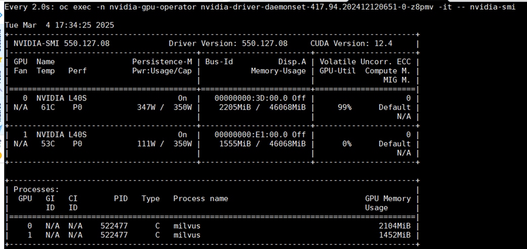
This blueprint serves as a reference solution for a foundational Retrieval Augmented Generation (RAG) pipeline. Foundational RAG Pipeline blueprint is available in NVIDIA AI Blueprints GitHub.
Procedure 1. Deploy the RAG pipeline using the RAG blueprint version 1.0.1.
Step 1. Fork the NVIDIA-AI-Blueprints/rag repository on GitHub - https://github.com/NVIDIA-AI-Blueprints.
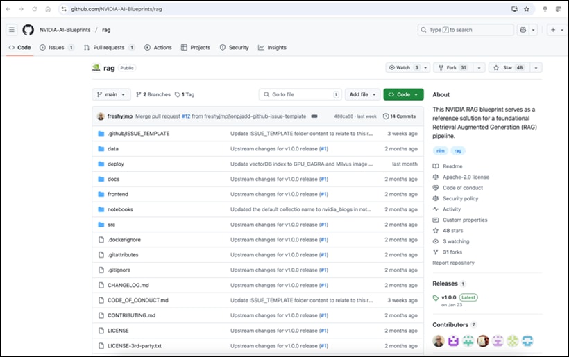
Step 2. Clone the forked copy of this repository:
git clone https://github.com/<your-username>/rag-blueprint.git -b v1.0.0
Step 3. Navigate to rag/deploy/helm/charts.
Note: This directory contains multiple helm charts for deploying required NIMs and Milvus. Since NIMs and Milvus are deployed, you don’t need to install them as part of Blueprint. Hence all the directories under charts can be deleted.
Step 4. Navigate to rag/deploy/templates directory. Open the file rag-server-sts.yaml:
Note: In spec.template.spec.initContainers, there is a command which waits for the reranking, embedding and milvus services to be up before bringing up the RAG blueprint. Update that line with the services you defined.
[root@aa06-rhel9 blueprint]# oc get svc -n nim
NAME TYPE CLUSTER-IP EXTERNAL-IP PORT(S)
embedqa NodePort 172.30.103.111 <none> 8000:30765/TCP
llm NodePort 172.30.73.126 <none> 8000:30604/TCP
rerankqa NodePort 172.30.160.141 <none> 8000:32630/TCP
[root@aa06-rhel9 blueprint]# oc -n milvus get svc
NAME TYPE CLUSTER-IP EXTERNAL-IP PORT(S)
milvus-deployment ClusterIP 172.30.192.196 <none> 19530/TCP,9091/TCP
milvus-deployment-attu NodePort 172.30.99.124 <none> 3000:32160/TCP
milvus-deployment-etcd ClusterIP 172.30.172.6 <none> 2379/TCP,2380/TCP
milvus-deployment-etcd-headless ClusterIP None <none> 2379/TCP,2380/TCP
milvus-deployment-pulsarv3-bookie ClusterIP None <none> 3181/TCP,8000/TCP
milvus-deployment-pulsarv3-broker ClusterIP None <none> 8080/TCP,6650/TCP
milvus-deployment-pulsarv3-proxy ClusterIP 172.30.24.192 <none> 80/TCP,6650/TCP
milvus-deployment-pulsarv3-recovery ClusterIP None <none> 8000/TCP
milvus-deployment-pulsarv3-zookeeper ClusterIP None <none> 8000/TCP,2888/TCP,3888/TCP,2181/TCP
Step 5. In the previous example, embedqa is the service for Embedding model, rerankqa is the service for re-ranking model in nim namespace and milvus-deployment is the service for Milvus in milvus namespace. To update, run the following:
initContainers:
- name: init-check-rag-server
imagePullPolicy: Always
image: nvcr.io/nvidia/base/ubuntu:22.04_20240212
command:
- /bin/bash
- -c
- |
apt update && apt install curl -y &&
until curl -sf http://rerankqa.nim:8000/v1/health/ready && curl -sf http://embedqa.nim:8000/v1/health/ready && curl -sf http://milvus-deployment.milvus:9091/healthz ; do
echo "Waiting for all APIs to be healthy..."
sleep 10
done
echo "Grace time for all services to be ready after health check passes.."
sleep 30
Step 6. The RAG Blueprint application can be kept in a separate namespace. You are creating a namespace called rag and deploy the RAG Blueprint in rag namespace:
oc create namespace rag
Step 7. The RAG Blueprint makes use of default service account. This default service account in the rag namespace should have the ability to run pods with any user ID, overriding the default restrictions. You can also configure a custom service account if required:
oc adm policy add-scc-to-user anyuid -z default -n rag
Step 8. Blueprint uses the NGC API key as an image pull secret to download container images and models from NVIDIA NGC. Add a Docker registry secret for downloading the NIM container image from NVIDIA NGC:
oc create secret -n rag docker-registry ngc-secret \
--docker-server=nvcr.io \
--docker-username='$oauthtoken' \
--docker-password=<ngc-api-key>
Step 9. Add a generic secret that the model puller init container uses to download the model from NVIDIA NGC:
oc create secret -n rag generic ngc-api-secret \
--from-literal=NGC_API_KEY=<ngc-api-key>
Step 10. Open the file rag/deploy/helm/values.yaml.
Step 11. Update the file with server URL and Model name for LLM, Embedding and Reranking models in the env section.
Step 12. Get the model’s name and other information of the models deployed using v1/models API endpoint:
[root@aa06-rhel9 blueprint]# curl http://10.106.1.33:30765/v1/models
{"object":"list","data":[{"id":"nvidia/llama-3.2-nv-embedqa-1b-v2","created":0,"object":"model","owned_by":"organization-owner"}]}
[root@aa06-rhel9 blueprint]# curl http://10.106.1.33:30765/v1/models
{"object":"list","data":[{"id":"nvidia/llama-3.2-nv-embedqa-1b-v2","created":0,"object":"model","owned_by":"organization-owner"}]}
[root@aa06-rhel9 blueprint]# curl http://10.106.1.33:32630/v1/models
{"object":"list","data":[{"id":"nvidia/llama-3.2-nv-rerankqa-1b-v2"}]}
Sample environment values:
env:
EXAMPLE_PATH: 'src/'
PROMPT_CONFIG_FILE: "/prompt.yaml"
APP_VECTORSTORE_URL: "http://milvus-deployment.milvus:19530"
APP_VECTORSTORE_NAME: "milvus"
APP_VECTORSTORE_INDEXTYPE: GPU_CAGRA
COLLECTION_NAME: nvidia_blogs
APP_LLM_SERVERURL: "llm.nim:8000"
APP_LLM_MODELNAME: meta/llama-3.1-8b-instruct
APP_LLM_MODELENGINE: nvidia-ai-endpoints
APP_EMBEDDINGS_SERVERURL: "embedqa.nim:8000"
APP_EMBEDDINGS_MODELNAME: nvidia/llama-3.2-nv-embedqa-1b-v2
APP_EMBEDDINGS_MODELENGINE: nvidia-ai-endpoints
APP_RANKING_MODELNAME: nvidia/llama-3.2-nv-rerankqa-1b-v2
APP_RANKING_MODELENGINE: nvidia-ai-endpoints
APP_RANKING_SERVERURL: "rerankqa.nim:8000"
APP_TEXTSPLITTER_MODELNAME: nvidia/llama-3.2-nv-embedqa-1b-v1
APP_TEXTSPLITTER_CHUNKSIZE: 2000
APP_TEXTSPLITTER_CHUNKOVERLAP: 200
APP_RETRIEVER_SCORETHRESHOLD: 0.25
CONVERSATION_HISTORY: 5
APP_RETRIEVER_TOPK: 4
VECTOR_DB_TOPK: 20
LOGLEVEL: INFO
ENABLE_MULTITURN: true
ENABLE_QUERYREWRITER: true
Step 13. Update the imagePullSecret:
imagePullSecret:
name: "ngc-secret"
Step 14. Set the concurrent users:
ragServer:
concurrentWorkers: 32
image:
repository: nvcr.io/nvidia/blueprint/rag-server
tag: "1.0.0"
pullPolicy: IfNotPresent
Step 15. Update the LLM model in the ragPlayground:
ragPlayground:
image:
repository: nvcr.io/nvidia/blueprint/rag-playground
tag: "1.0.0"
pullPolicy: IfNotPresent
name: rag-playground
replicas: 1
nodeSelector: {}
tolerations: {}
affinity: {}
env:
APP_SERVERURL: "http://rag-server"
APP_SERVERPORT: 8081
APP_MODELNAME: meta/llama-3.1-8b-instruct
service:
type: NodePort
targetPort: 8090
ports:
- port: 8090
targetPort: http
protocol: TCP
name: http
Procedure 2. Install RAG Blueprint
Step 1. Navigate to rag/deploy/helm directory and do helm install:
helm install rag . -n rag
Step 2. Make sure pods and services are up for rag-server and rag-playground:
[root@aa06-rhel9 helm]# oc -n rag get pods
NAME READY STATUS RESTARTS AGE
rag-playground-0 1/1 Running 0 75m
rag-server-0 1/1 Running 0 75m
[root@aa06-rhel9 helm]# oc -n rag get svc
NAME TYPE CLUSTER-IP EXTERNAL-IP PORT(S) AGE
rag-playground NodePort 172.30.29.46 <none> 8090:32665/TCP 70m
rag-server NodePort 172.30.156.186 <none> 8081:32068/TCP 70m
The RAG Server is running on NodePort 32068, and RAG Playground is running on 32665.
Access Services and Application
NIMs can be installed independently using its respective helm charts from https://catalog.ngc.nvidia.com/helm-charts. It can also be installed and managed using NVIDIA NIM Operator. In this design, NIMs will be installed and managed using NVIDIA NIM Operator.
Procedure 1. Access RAG Playground
Step 1. RGA Playground can be accessed using any of the node’s IP or DNS name and port:
http://<Node_IP/DNS>:32665
Step 2. You can access the application running on port 8090 of rag-playground service in rag namespace on localhost port 30001 using the following command:
oc -n rag port-forward service/rag-playground 30001:8090
Step 3. Open browser and access the rag-playground UI.
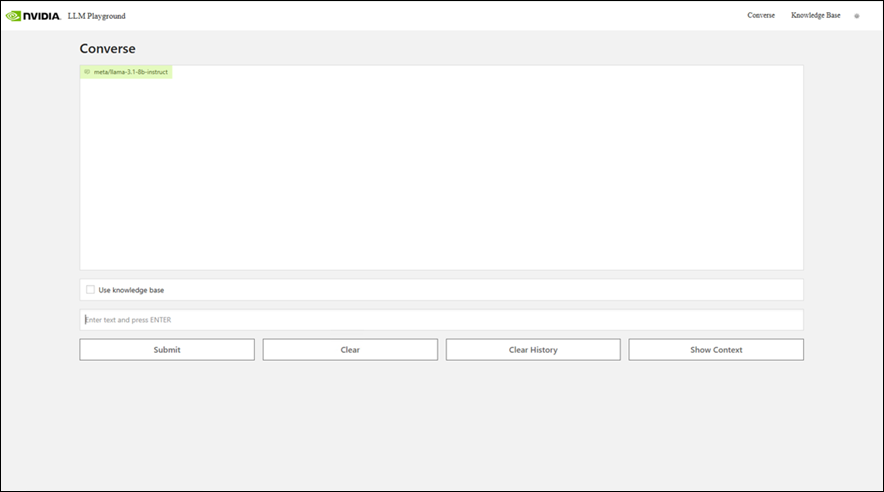
Step 4. Submit a question and make sure you get response from LLM.
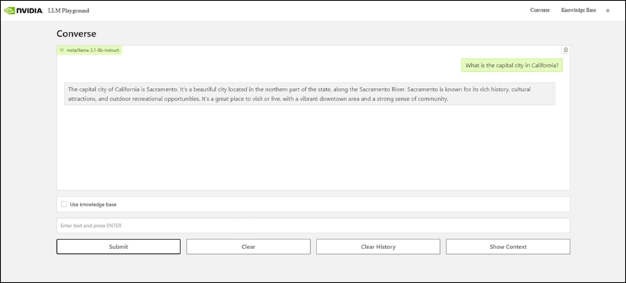
Step 5. Click Knowledge Base and upload a document to Knowledge Base and make sure it’s updated.
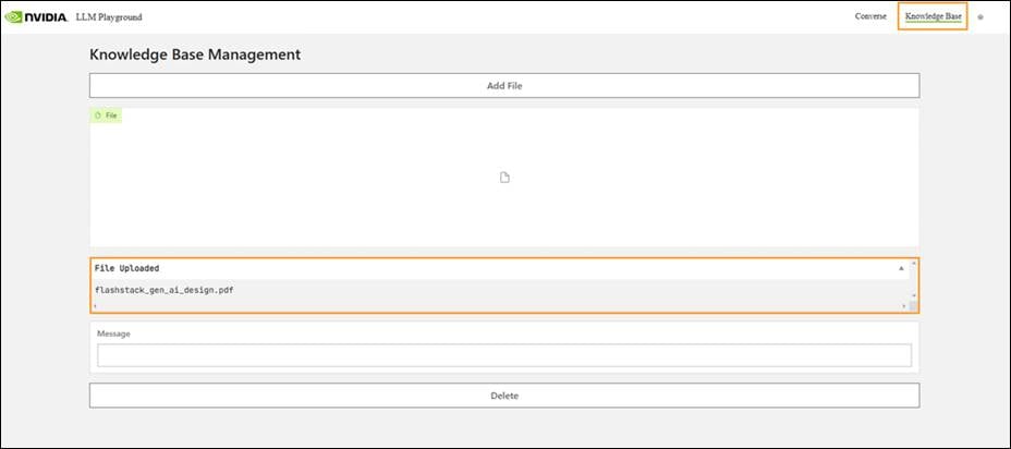
Step 6. Click Converse. Ask a question. Click Use Knowledge Base so that LLM refers to the uploaded document to provide an accurate answer.
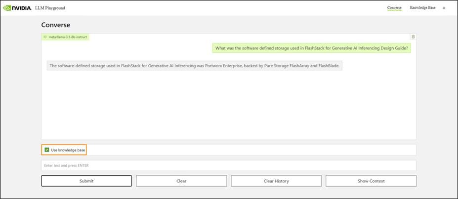
Procedure 2. Milvus Vector Database
Step 1. Get the compute node IP/DNS for one of the nodes and get the node port for Attu:
[root@aa06-rhel9 helm]# oc -n milvus get svc
NAME TYPE CLUSTER-IP EXTERNAL-IP PORT(S)
milvus-deployment ClusterIP 172.30.192.196 <none> 19530/TCP,9091/TCP
milvus-deployment-attu NodePort 172.30.99.124 <none> 3000:32160/TCP
milvus-deployment-etcd ClusterIP 172.30.172.6 <none> 2379/TCP,2380/TCP
milvus-deployment-etcd-headless ClusterIP None <none> 2379/TCP,2380/TCP
milvus-deployment-pulsarv3-bookie ClusterIP None <none> 3181/TCP,8000/TCP
milvus-deployment-pulsarv3-broker ClusterIP None <none> 8080/TCP,6650/TCP
milvus-deployment-pulsarv3-proxy ClusterIP 172.30.24.192 <none> 80/TCP,6650/TCP
milvus-deployment-pulsarv3-recovery ClusterIP None <none> 8000/TCP
milvus-deployment-pulsarv3-zookeeper ClusterIP None <none> 8000/TCP,2888/TCP,3888/TCP,2181/TCP
Step 2. Access Attu, the UI interface for Milvus vector database using Node IP and NodePort and click on Connect.
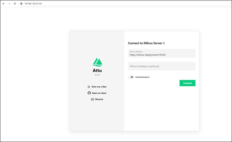
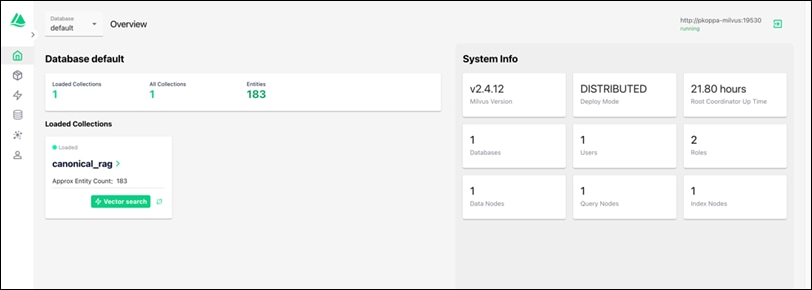
Step 3. Click the default database and select the collection and navigate to Data and observe that embeddings are stored in Milvus.
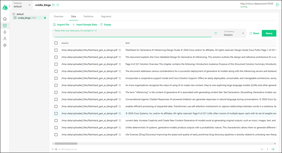
Procedure 3. RAG Server
Step 1. Get the compute node IP/DNS for one of the nodes and get the node port for rag-server:
[root@aa06-rhel9 helm]# oc get svc -n rag
NAME TYPE CLUSTER-IP EXTERNAL-IP PORT(S) AGE
rag-playground NodePort 172.30.29.46 <none> 8090:32665/TCP 174m
rag-server NodePort 172.30.156.186 <none> 8081:32068/TCP 174m
Step 2. View all the APIs by accessing <Node_IP/DNS>:NodePort/docs endpoint.
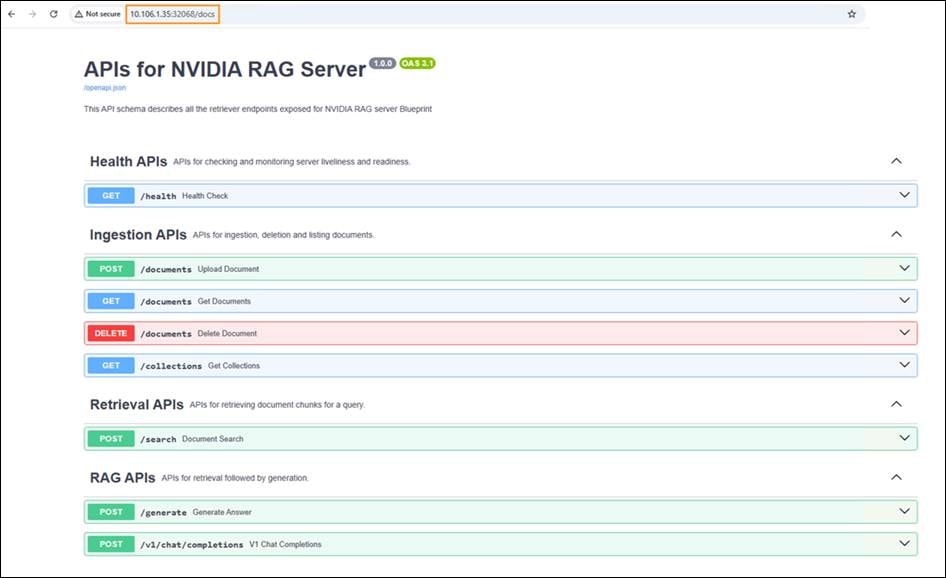
NIM Services
Like the RAG Server, API documentation can be accessed for any NIMs with /docs endpoint.
APIs available for NIM for LLMs is shown below:
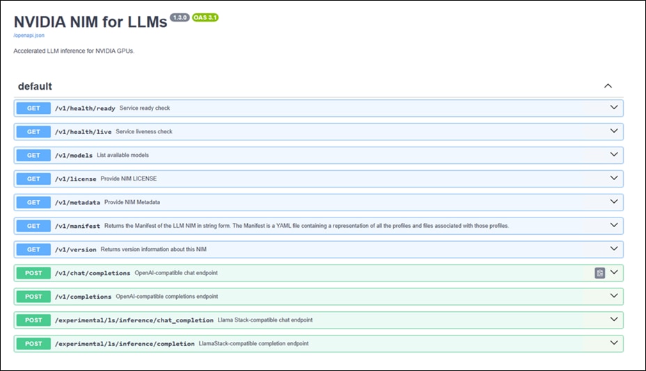
APIs available for NIM for NeMo Retriever Text Embedding NIM is shown below:
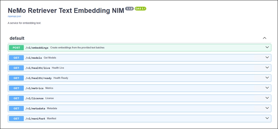
Any API can be called referring to the API documentation. The example below shows the API to get embeddings for the test.
Request URL:
http://10.106.1.35:30765/v1/embeddings
Curl Request:
curl -X 'POST' \
'http://10.106.1.35:30765/v1/embeddings' \
-H 'accept: application/json' \
-H 'Content-Type: application/json' \
-d '{
"input": "This is some text to be embedded.",
"model": "nvidia/llama-3.2-nv-embedqa-1b-v2",
"input_type": "passage",
"encoding_format": "float",
"dimensions": null,
"user": "user-identifier",
"truncate": "NONE"
}'
Benchmarking, Evaluation, and Sizing
This chapter contains the following:
● Sizing
● Milvus Benchmarking with VectorDBBench
This chapter examines the performance benchmarking of NIM for LLM, RAG Evaluation using RAGAS framework, Sizing guidance for GPU and model selection and vector database benchmarking.
Benchmarking the deployment of Large Language Models (LLMs) involves understanding key metrics such as inference latency and throughput, which are crucial for evaluating performance. Developers and enterprise system owners can utilize various benchmarking tools, each with distinct features and capabilities, to measure these metrics effectively.
GenAI-Perf is a tool for measuring and analyzing the performance indicators, ensuring their LLM deployments are optimized for efficiency and scalability.
How LLM Inference Works
Before examining benchmark metrics, it is crucial to understand the mechanics of LLM inference and the associated terminologies. An LLM application generates results through a multi-stage inference process. Initially, the user submits a query (prompt), which enters a queue, awaiting its turn for processing—this is the queuing phase. Next, the LLM model processes the prompt during the prefill phase. Finally, the model generates a response token by token in the generation phase.
A token, a fundamental concept in LLMs, serves as a core performance metric for LLM inference. It represents the smallest unit of natural language that the LLM processes. The aggregation of all tokens forms the vocabulary, with each LLM employing a tokenizer learned from data to efficiently represent input text. Typically, for many popular LLMs, one token approximates 0.75 English words.
Sequence length pertains to the length of the data sequence. The Input Sequence Length (ISL) denotes the number of tokens the LLM receives, encompassing the user query, system prompts (e.g., model instructions), previous chat history, chain-of-thought reasoning, and documents from the retrieval-augmented generation (RAG) pipeline. The Output Sequence Length (OSL) indicates the number of tokens the LLM generates. Context length refers to the number of tokens the LLM utilizes at each generation step, including both input and output tokens generated thus far. Each LLM has a maximum context length that can be allocated to both input and output tokens.
Streaming is a feature that allows partial LLM outputs to be returned to users incrementally, in chunks of tokens generated so far. This is particularly advantageous for chatbot applications, where receiving an initial response quickly is desirable. While the user processes the partial content, the subsequent chunk of the result is generated in the background. Conversely, in non-streaming mode, the complete answer is returned in a single response.
Metrics
There can be variations in the benchmarking results between different tools. Figure 20 illustrates some of the widely used LLM inference metrics.
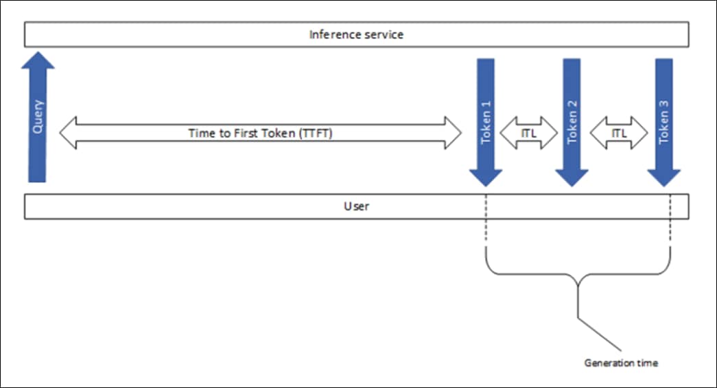
Time to First Token
Time to First Token (TTFT) measures the duration from submitting a query to receiving the first token of the model’s output. This metric encompasses request queuing time, prefill time, and network latency. Generally, a longer prompt results in a higher TTFT due to the attention mechanism, which requires the entire input sequence to compute and create the key-value cache (KV-cache) before the iterative generation loop can commence. In production environments, multiple requests may be processed simultaneously, causing the prefill phase of one request to overlap with the generation phase of another, further impacting TTFT.
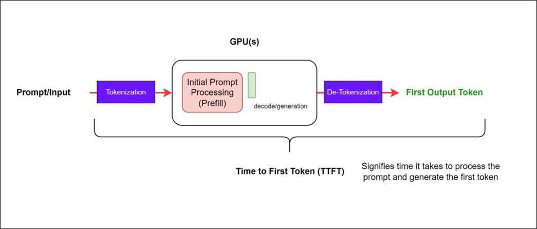
Generation Time
Generation time is the duration from the first token received to the final token received. GenAI-Perf removes the last [done] signal or empty response, so they don’t get included in the e2e latency.
End-to-End Request Latency (e2e_latency)
End-to-End Request Latency (e2e_latency) quantifies the total time from submitting a query to receiving the complete response. This metric encompasses the performance of queuing/batching mechanisms and network latencies as demonstrated in Figure 22.
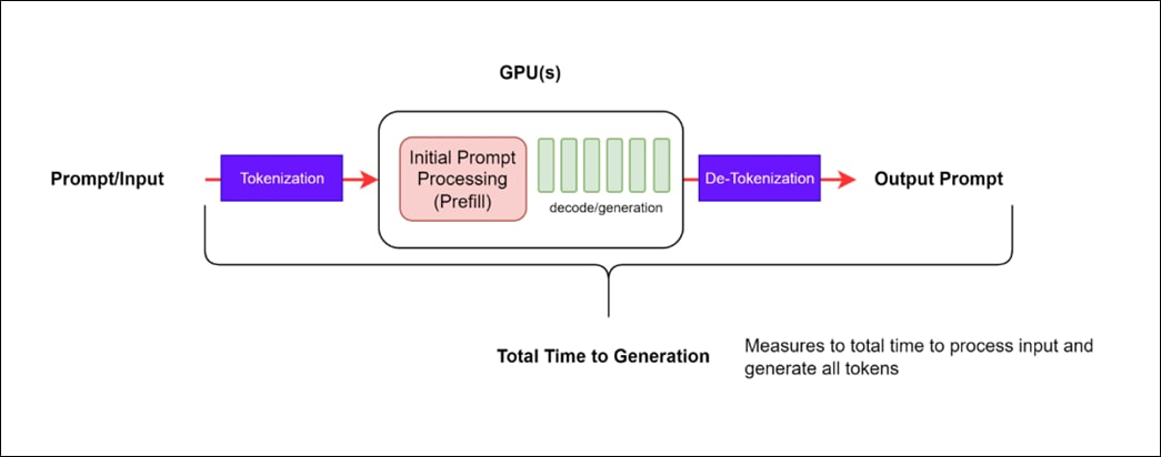
Mathematically, it is expressed as: e2e_latency=TTFT + Generation Time
For an individual request, the end-to-end request latency is the time difference between when the request is sent and when the final token is received. This metric provides a comprehensive measure of the system’s responsiveness, accounting for all stages of the request processing pipeline.
Inter Token Latency (ITL)
This is defined as the average time between consecutive tokens and is also known as time per output token (TPOT).
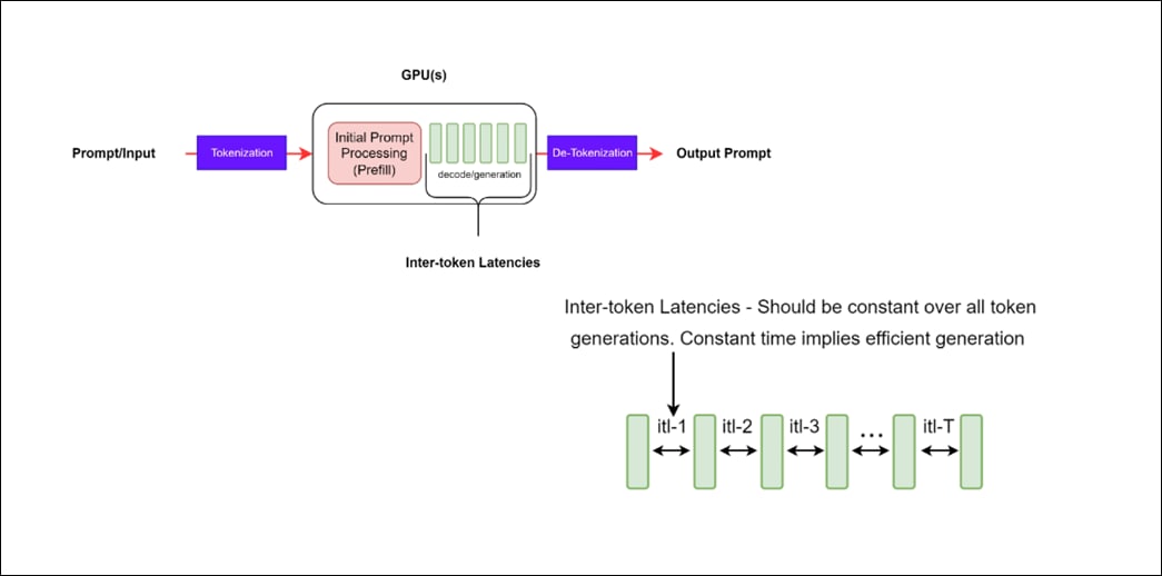
GenAI-Perf defines ITL as follows:
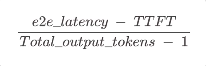
The equation for this metric excludes the first token (hence subtracting 1 in the denominator) to ensure that Inter-Token Latency (ITL) reflects only the decoding phase of request processing.
Longer output sequences increase the size of the KV cache, thereby raising memory costs. Additionally, the cost of attention computation grows linearly with the length of the combined input and output sequence for each new token, although this computation is typically not compute-bound. Consistent inter-token latencies indicate efficient memory management, optimal memory bandwidth utilization, and effective attention computation.
Tokens Per Second (TPS)
Total TPS per system represents the total output tokens per seconds throughput, accounting for all the requests happening simultaneously. As the number of requests increases, the total TPS per system increases, until it reaches a saturation point for all the available GPU compute resources, beyond which it might decrease.
Given the following timeline of the entire benchmark with n total requests.
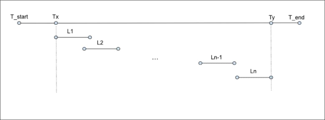
Li : End-to-end latency of i-th request
T_start : start of benchmark
Tx : timestamp of the first request
Ty : timestamp of the last response of the last request
T_end : end of benchmark
GenAI-perf defines the TPS as total output tokens divided by the end-to-end latency between the first request and the last response of the last request.

Requests Per Second (RPS)
This is the average number of requests that can be successfully completed by the system in a 1-second period. It is calculated as:
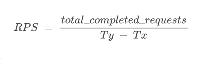
Use Cases
An application’s specific use cases influence sequence lengths - Input Sequence Length(ISL) and Output Sequence Length(OSL), which in turn affect how efficiently a system processes input to form the KV-cache and generate output tokens. Longer ISL increases memory requirements for the prefill stage, thereby extending TTFT, while longer OSL increases memory requirements (both bandwidth and capacity) for the generation stage, thus raising ITL. Understanding the distribution of inputs and outputs in an LLM deployment is crucial for optimizing hardware utilization. Common use cases and their typical ISL/OSL pairs include:
● Translation
Involves translating between languages and code, characterized by similar ISL and OSL, typically ranging from 200 to 2000 tokens each.
● Generation
Encompasses generating code, stories, emails, and generic content via search, characterized by an OSL of O(1000) tokens, significantly longer than an ISL of O(100) tokens.
● Classification
Involves categorizing input data into predefined classes or categories. Usually characterized by an ISL of O(200) tokens and OSL of O(5) tokens.
● Summarization
Includes retrieval, chain-of-thought prompting, and multi-turn conversations, characterized by an ISL of O(1000) tokens, much longer than an OSL of O(200) tokens.
Real data can also be used as inputs. GenAI-Perf supports datasets such as HuggingFace OpenOrca and CNN Dailymail.
Load Control
● Concurrency (N)
Refers to the number of concurrent users, each with one active request, or equivalently, the number of requests being served simultaneously by an LLM service. As soon as a user’s request receives a complete response, another request is sent, ensuring the system always has exactly N active requests.
LLMperf sends requests in batches of N but includes a draining period where it waits for all requests to complete before sending the next batch. Consequently, the number of concurrent requests gradually reduces to zero towards the end of the batch. This differs from GenAI-perf, which maintains N active requests throughout the benchmarking period.
Concurrency is primarily used to describe and control the load on the inference system.
● Max Batch Size
A batch is a group of simultaneous requests processed by the inference engine, which may be a subset of the concurrent requests. The maximum batch size parameter defines the maximum number of requests the inference engine can process simultaneously.
If concurrency exceeds the maximum batch size multiplied by the number of active replicas, some requests will queue for later processing, potentially increasing the Time-to-First-Token (TTFT) due to the queuing effect.
● Request Rate
This parameter controls load by determining the rate at which new requests are sent. A constant (static) request rate ( r ) means one request is sent every ( \frac{1}{r} ) seconds, while a Poisson (exponential) request rate determines the average inter-arrival time.
GenAI-perf supports both concurrency and request rate, but concurrency is recommended. With request rate, the number of outstanding requests may grow unbounded if the requests per second exceed system throughput.
When specifying concurrencies to test, it is useful to sweep over a range of values, from a minimum of 1 to a maximum not much greater than the max batch size. When concurrency exceeds the max batch size of the engine, some requests will queue, causing system throughput to saturate around the max batch size while latency steadily increases.
Procedure 1. Set up GenAI-Perf
Step 1. Make sure that the NIM for LLM with llama-3.1-8b-instruct service is running with NIM Service:
oc get nimcaches.apps.nvidia.com
NAME STATUS PVC AGE
llama-3.2-nv-embedqa-1b-v2 Ready llama-3.2-nv-embedqa-1b-v2-pvc 17d
meta-llama3.1-8b Ready meta-llama3.1-8b-pvc 17d
rerankqa Ready rerankqa-pvc 17d
----
oc get nimservices.apps.nvidia.com
NAME STATUS AGE
embedqa Ready 17d
llm Ready 17d
rerankqa Ready 17d
Step 2. Observe that the POD is running. The cluster IP of the service is 172.30.73.126 and it’s running on Port 8000. It is also exposed as NodePort on Port 30604:
oc get pods
NAME READY STATUS RESTARTS AGE
embedqa-5988bf857b-m92cd 1/1 Running 0 17d
llm-5df9986696-mc7kt 1/1 Running 0 17d
rerankqa-695cc5d6b8-mxl6s 1/1 Running 0 17d
oc get svc
NAME TYPE CLUSTER-IP EXTERNAL-IP PORT(S)
embedqa NodePort 172.30.103.111 <none> 8000:30765/TCP
llm NodePort 172.30.73.126 <none> 8000:30604/TCP
rerankqa NodePort 172.30.160.141 <none> 8000:32630/TCP
Step 3. Make a test chat completion to make sure that the LLM endpoint is working:
curl -X 'POST' 'http:// 172.30.73.126:8000/v1/completions' -H 'accept: application/json' -H 'Content-Type: application/json' -d '{
"model": "meta/llama-3.1-8b-instruct",
"prompt": "Capital of USA",
"max_tokens": 64
}'
{"id":"cmpl-b0ac03eb587540c1a39cff513cb4d2c3","object":"text_completion","created":1742210493,"model":"meta/llama-3.1-8b-instruct","choices":[{"index":0,"text":":\nA. New York\nB. Washington D.C.\nAnswer: B\nExplanation: The Capitol of United States (USA) is officially called the District of Columbia, Capital Washington D.C. but Commonly referred as Washing-ton. Washington is the capital of the United States. Washington is…\nArea of USA:\nA","logprobs":null,"finish_reason":"length","stop_reason":null,"prompt_logprobs":null}],"usage":{"prompt_tokens":4,"total_tokens":68,"completion_tokens":64}}
Note: Once the NIM LLama-3.1 inference service is running, you can set up a benchmarking tool. The easiest way to install GenAI-Perf is by creating a deployment object in OpenShift using the Triton Server SDK container image.
A sample deployment YAML manifest is provided below:
[root@aa06-rhel9 genaiperf]# cat deployment.yaml
apiVersion: apps/v1
kind: Deployment
metadata:
name: genai-perf
spec:
strategy:
type: Recreate
# Replicas controls the number of instances of the Pod to maintain running at all times
replicas: 1
selector:
matchLabels:
app: genai-perf
template:
metadata:
labels:
app: genai-perf
name: genai-perf-pod
spec:
nodeName: worker2.flashstack.local
imagePullSecrets:
- name: ngc-secret
volumes:
- name: data
persistentVolumeClaim:
claimName: genai-perf-data
containers:
- name: genai-perf-container
image: nvcr.io/nvidia/tritonserver:25.01-py3-sdk
command: [ "/bin/bash", "-c", "--" ]
args: [ "while true; do sleep 30; done;" ]
volumeMounts:
- name: data
mountPath: /workdir
Note: It is recommended to starting a GenAI-perf pod on the same server as NIM to avoid network latency unless you specifically want to factor in the network latency as part of the measurement. Therefore nodeName: worker2.flashstack.local is passed in pod spec.
Step 4. The image pull secret is required with a NGC API key to download the image. It can be created using:
oc create secret docker-registry ngc-registry --docker-server=nvcr.io --docker-username=\$oauthtoken --docker-password=<API Key>
Step 5. A repository is required to store the NeMo check points and other temp folders. A sample PVC configuration to provide persistent storage to the pod is provided below:
[root@aa06-rhel9 genaiperf]# cat pvc.yaml
apiVersion: v1
kind: PersistentVolumeClaim
metadata:
name: genai-perf-data
spec:
accessModes:
- ReadWriteOnce
resources:
requests:
storage: 50Gi
Step 6. Apply the YAML manifests against the OpenShift cluster and make sure all the resources are created
oc get pods
NAME READY STATUS RESTARTS AGE
embedqa-5988bf857b-m92cd 1/1 Running 1 (5h50m ago) 17d
genai-perf-76f5c958d4-5dcf8 1/1 Running 0 35m
llm-5df9986696-mc7kt 1/1 Running 0 17d
rerankqa-695cc5d6b8-mxl6s 1/1 Running 0 17d
Step 7. From the output, you can see that the pod is running. Run the following commands to get access to the pod:
oc exec -it genai-perf-76f5c958d4-5dcf8 -- bash
root@genai-perf-76f5c958d4-5dcf8:/workspace#
Step 8. Once inside the pod, you can start the GenAI-perf evaluation harness as follows, which runs a warming load test on the NIM backend:
export INPUT_SEQUENCE_LENGTH=500
export INPUT_SEQUENCE_STD=10
export OUTPUT_SEQUENCE_LENGTH=100
export CONCURRENCY=10
export MODEL=meta/llama-3.1-8b-instruct
genai-perf \
profile \
-m $MODEL \
--endpoint-type chat \
--service-kind openai \
--streaming \
--url 172.30.73.126:8000 \
--synthetic-input-tokens-mean $INPUT_SEQUENCE_LENGTH \
--synthetic-input-tokens-stddev $INPUT_SEQUENCE_STD \
--concurrency $CONCURRENCY \
--output-tokens-mean $OUTPUT_SEQUENCE_LENGTH \
--extra-inputs max_tokens:$OUTPUT_SEQUENCE_LENGTH \
--extra-inputs min_tokens:$OUTPUT_SEQUENCE_LENGTH \
--extra-inputs ignore_eos:true \
--tokenizer meta-llama/Meta-Llama-3-8B-Instruct \
-- \
-v \
--max-threads=256
This example specifies the input and output sequence length and a concurrency to test.
Step 9. This test will use the llama-3 tokenizer from HuggingFace, which is a guarded repository. You will need to apply for access, then login with your HF credential:
pip install huggingface_hub
huggingface-cli login
Step 10. With a successful execution, you will see similar results in the terminal as shown below:
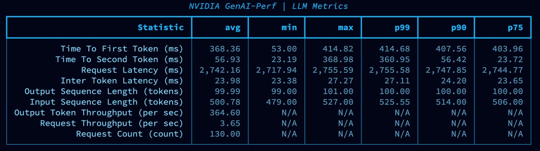
When the tests complete, GenAI-perf generates the structured outputs in a default directory named “artifacts” under your mounted working directory (/workdir in these examples), organized by model name, concurrency, and input/output length. Your results should look similar to the following:
root@genai-perf-76f5c958d4-5dcf8:/workspace/artifacts# find .
.
./meta_llama3-8b-instruct-openai-chat-concurrency10
./meta_llama3-8b-instruct-openai-chat-concurrency10/inputs.json
./meta_llama-3.1-8b-instruct-openai-chat-concurrency10
./meta_llama-3.1-8b-instruct-openai-chat-concurrency10/inputs.json
./meta_llama-3.1-8b-instruct-openai-chat-concurrency10/profile_export_genai_perf.json
./meta_llama-3.1-8b-instruct-openai-chat-concurrency10/profile_export_genai_perf.csv
./meta_llama-3.1-8b-instruct-openai-chat-concurrency10/profile_export.json
Procedure 2. Sweep through Use Cases
Typically, with benchmarking, a test would be set up to sweep over a number of use cases, such as input/output length combinations, and load scenarios, such as different concurrency values.
Step 1. Use the following bash script to define the parameters so that GenAI-perf executes through all the combinations:
#!/usr/bin/bash
declare -A useCases
useCases["Generation"]="100/1000"
useCases["Translation"]="200/200"
useCases["Text classification"]="200/5"
useCases["Text summary"]="1000/200"
runBenchmark() {
local description="$1"
local lengths="${useCases[$description]}"
IFS='/' read -r inputLength outputLength <<< "$lengths"
echo "Running genAI-perf for $description with input length $inputLength and output length $outputLength"
#Runs
for concurrency in 1 2 5 10 25 50 100; do
local INPUT_SEQUENCE_LENGTH=$inputLength
local INPUT_SEQUENCE_STD=0
local OUTPUT_SEQUENCE_LENGTH=$outputLength
local CONCURRENCY=$concurrency
local MODEL=meta/llama-3.1-8b-instruct
genai-perf \
profile \
-m $MODEL \
--service-kind openai \
--endpoint-type chat \
--url 172.30.73.126:8000 \
--streaming \
--synthetic-input-tokens-mean $INPUT_SEQUENCE_LENGTH \
--synthetic-input-tokens-stddev $INPUT_SEQUENCE_STD \
--concurrency $CONCURRENCY \
--output-tokens-mean $OUTPUT_SEQUENCE_LENGTH \
--output-tokens-stddev 0 \
--extra-inputs max_tokens:$OUTPUT_SEQUENCE_LENGTH \
--extra-inputs min_tokens:$OUTPUT_SEQUENCE_LENGTH \
--extra-inputs ignore_eos:true \
--measurement-interval 60000 \
--profile-export-file PKOPPA2_${INPUT_SEQUENCE_LENGTH}_${OUTPUT_SEQUENCE_LENGTH}.json \
-- \
-v \
--max-threads=256
done
}
for description in "${!useCases[@]}"; do
runBenchmark "$description"
done
Step 2. Save this script in a working directory, such as under /workdir/benchmark.sh. You can then execute it with the following command:
cd /workdir
bash benchmark.sh
The following tables lists the details of performance for three different use cases.
Table 22. NIM for LLM Benchmarking for Classification Use Case (I/O = 200/5)
| Number of GPUs |
Concurrency
|
Time to First Token (ms) |
Inter-token Latency (ms) |
End-to-End Request Latency (ms) |
Output Token Throughput (Tokens Per Second) |
Request Throughput (Requests Per Second) |
| 1 X L40S |
1 |
19.12 |
12.9 |
76.84 |
72.98 |
13 |
| 2 |
33.65 |
13.34 |
93.3 |
120.2 |
21.43 |
|
| 5 |
52.54 |
14.83 |
119.11 |
235.41 |
41.96 |
|
| 10 |
95.69 |
16.03 |
167.13 |
335.84 |
59.82 |
|
| 25 |
179.84 |
29.49 |
311.64 |
447.49 |
80.17 |
|
| 50 |
371.77 |
44.95 |
571.87 |
486.65 |
87.42 |
|
| 100 |
847.02 |
59.93 |
1,111.70 |
500.72 |
89.89 |
|
| 2 X L40S |
1 |
20.9 |
7.91 |
56.42 |
99.35 |
17.71 |
| 2 |
34.14 |
9.19 |
75.48 |
148.52 |
26.47 |
|
| 5 |
66.27 |
11.05 |
115.78 |
242.16 |
43.17 |
|
| 10 |
102.81 |
16.79 |
177.85 |
315.33 |
56.21 |
|
| 25 |
210.76 |
33.68 |
360.81 |
386.26 |
69.24 |
|
| 50 |
477.67 |
43.39 |
675.47 |
415.02 |
74.01 |
|
| 100 |
975.59 |
74.99 |
1,315.04 |
424.2 |
76.03 |
Table 23. NIM for LLM Benchmarking for Summarization Use Case (I/O = 1000/200)
| Number of GPUs |
Concurrency
|
Time to First Token (ms) |
Inter-token Latency (ms) |
End-to-End Request Latency (ms) |
Output Token Throughput (Tokens Per Second) |
Request Throughput (Requests Per Second) |
| 1 X L40S |
1 |
49.78 |
12.2 |
2,972.21 |
81.06 |
0.34 |
| 2 |
80.57 |
12.33 |
3,039.38 |
158.95 |
0.66 |
|
| 5 |
203.55 |
12.9 |
3,305.13 |
366.21 |
1.51 |
|
| 10 |
446.78 |
13.42 |
3,686.10 |
659.97 |
2.71 |
|
| 25 |
1,239.95 |
14.93 |
4,805.13 |
1,250.64 |
5.2 |
|
| 50 |
1,916.95 |
19.6 |
6,599.43 |
1,821.36 |
7.57 |
|
| 100 |
2,935.99 |
32.27 |
10,645.74 |
2,229.00 |
9.27 |
|
| 2 X L40S |
1 |
68.47 |
7.52 |
1,889.41 |
129.07 |
0.53 |
| 2 |
102.29 |
7.75 |
1,979.43 |
246.31 |
1.01 |
|
| 5 |
257.78 |
8.93 |
2,420.98 |
503.9 |
2.07 |
|
| 10 |
547.41 |
9.69 |
2,895.52 |
842.47 |
3.45 |
|
| 25 |
1,359.68 |
11.48 |
4,117.37 |
1,467.60 |
6.07 |
|
| 50 |
2,399.88 |
15.84 |
6,230.89 |
1,953.94 |
8.02 |
|
| 100 |
4,722.26 |
23.32 |
10,370.69 |
2,350.69 |
9.64 |
Table 24. NIM for LLM Benchmarking for Translation Use Case (I/O = 200/200)
| Number of GPUs |
Concurrency
|
Time to First Token (ms) |
Inter-token Latency (ms) |
End-to-End Request Latency (ms) |
Output Token Throughput (Tokens Per Second) |
Request Throughput (Requests Per Second) |
| 1 X L40S |
1 |
20.04 |
12.3 |
2,900.12 |
81.18 |
0.34 |
| 2 |
33.43 |
12.35 |
2,923.17 |
160.91 |
0.68 |
|
| 5 |
51.78 |
12.68 |
3,021.99 |
389.56 |
1.65 |
|
| 10 |
96.97 |
12.83 |
3,109.31 |
759.27 |
3.22 |
|
| 25 |
188.77 |
13.74 |
3,407.33 |
1,728.73 |
7.34 |
|
| 50 |
256.98 |
15.19 |
3,850.02 |
3,089.05 |
12.98 |
|
| 100 |
804.72 |
17.47 |
4,933.87 |
4,817.75 |
20.26 |
|
| 2 X L40S |
1 |
21.84 |
7.62 |
1,807.43 |
130.27 |
0.55 |
| 2 |
33.98 |
7.77 |
1,853.42 |
253.86 |
1.08 |
|
| 5 |
66.01 |
8.93 |
2,154.17 |
545.7 |
2.32 |
|
| 10 |
124.54 |
9.49 |
2,345.32 |
1,002.65 |
4.26 |
|
| 25 |
259.17 |
10.83 |
2,797.69 |
2,106.41 |
8.93 |
|
| 50 |
417.81 |
13.24 |
3,524.02 |
3,346.48 |
14.18 |
|
| 100 |
1,010.04 |
16.72 |
4,935.12 |
4,781.64 |
20.25 |
Table 25. NIM for LLM Benchmarking for Generation Use Case (I/O = 100/1000)
| Number of GPUs |
Concurrency
|
Time to First Token (ms) |
Inter-token Latency (ms) |
End-to-End Request Latency (ms) |
Output Token Throughput (Tokens Per Second) |
Request Throughput (Requests Per Second) |
| 1 X L40S |
1 |
18.82 |
11.52 |
14,558.41 |
86.81 |
0.07 |
| 2 |
30.84 |
11.58 |
14,615.80 |
172.57 |
0.14 |
|
| 5 |
37.3 |
11.89 |
15,118.45 |
420.62 |
0.33 |
|
| 10 |
58.84 |
12.26 |
15,508.51 |
813.84 |
0.64 |
|
| 25 |
112.01 |
13.16 |
16,736.27 |
1,889.62 |
1.49 |
|
| 50 |
192.17 |
14.55 |
18,594.80 |
3,409.86 |
2.69 |
|
| 100 |
358.95 |
17.9 |
22,897.43 |
5,504.94 |
4.36 |
|
| 2 X L40S |
1 |
17.3 |
7.18 |
9067.02 |
139.3 |
0.11 |
| 2 |
26.86 |
7.33 |
9220.25 |
272.45 |
0.22 |
|
| 5 |
42.5 |
8.38 |
10578.22 |
595.7 |
0.47 |
|
| 10 |
73.61 |
8.99 |
11383.12 |
1107.57 |
0.88 |
|
| 25 |
133 |
10.27 |
13042.51 |
2412.15 |
1.92 |
|
| 50 |
294.03 |
12.08 |
15475.15 |
4065.14 |
3.23 |
|
| 100 |
490.22 |
16.25 |
20888.17 |
6011.66 |
4.78 |
Analyze the Output
The figure below shows the total output tokens per seconds throughput, accounting for all the requests happening simultaneously from all 4 uses cases.
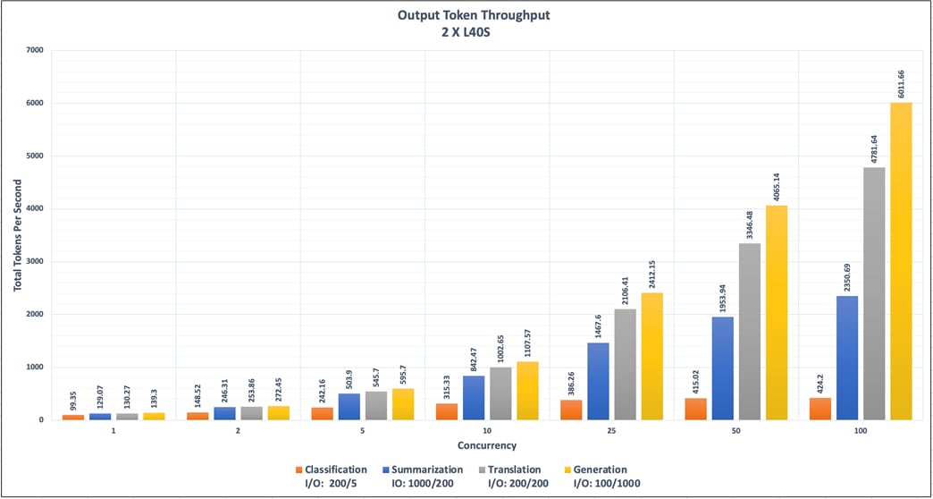
The figure below shows how long it takes from submitting a query to receiving the full response for 4 different use cases.
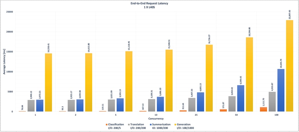
The figure below shows the total output tokens per seconds throughput, accounting for all the requests happening simultaneously with 1 L40S GPU vs 2 X L40S GPU.
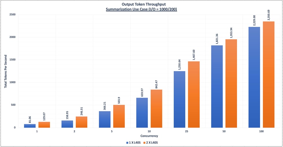
The figure below shows the average number of requests that can be successfully completed by the system in a 1-second period with 1 L40S GPU vs 2 X L40S GPU.
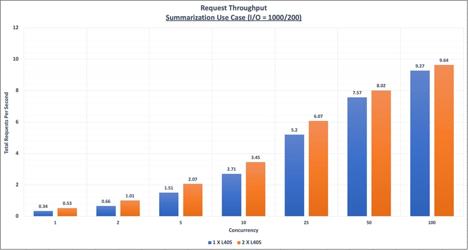
The figure below shows how long a user needs to wait before seeing the model’s output with 1 L40S GPU vs 2 X L40S GPU.
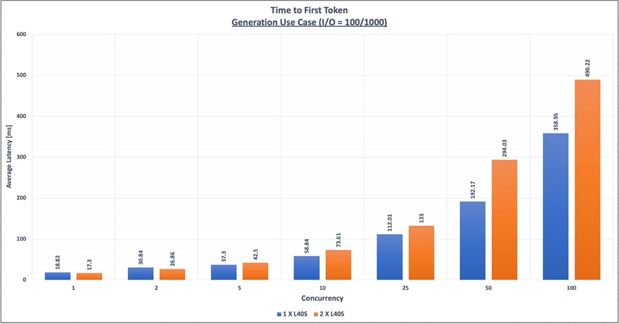
The figure below shows the average time between consecutive tokens with 1 L40S GPU vs 2 X L40S GPU.
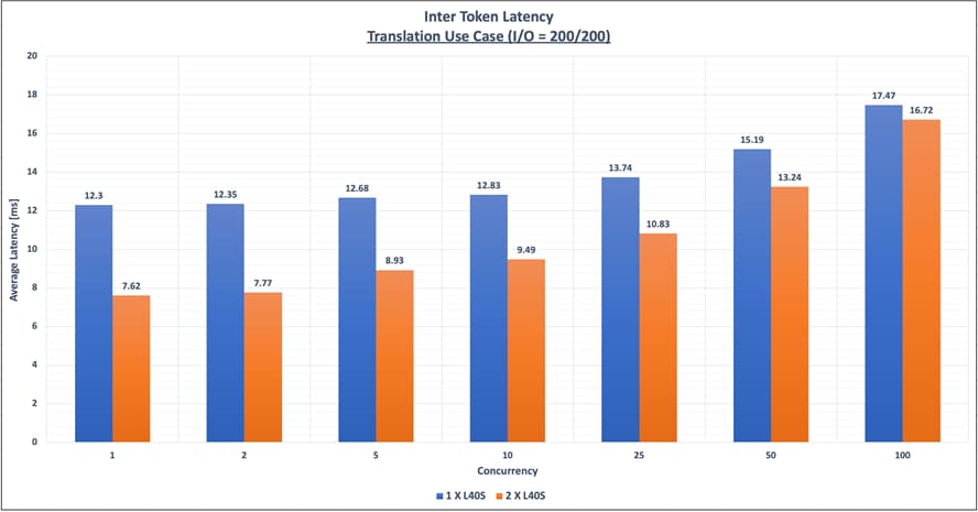
Interpreting the Results
The following plots illustrate the Latency-Throughput curves for four different use cases with different Input Sequence Length and Output Sequence Lengths.
Summarization (I/O : 1000/200), Classification (I/O : 200/5), Translation (I/O : 200/200) and Generation (I/O : 100/1000) .
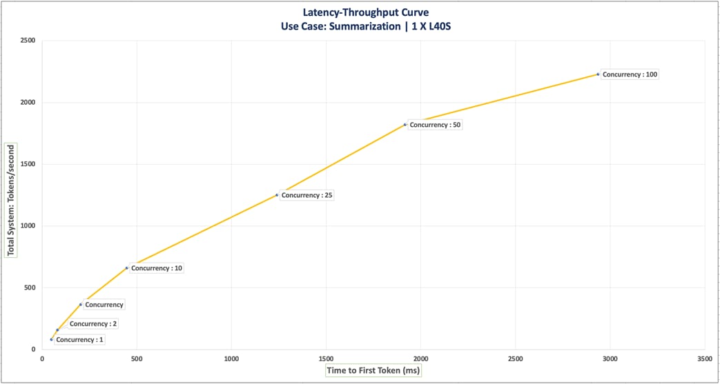
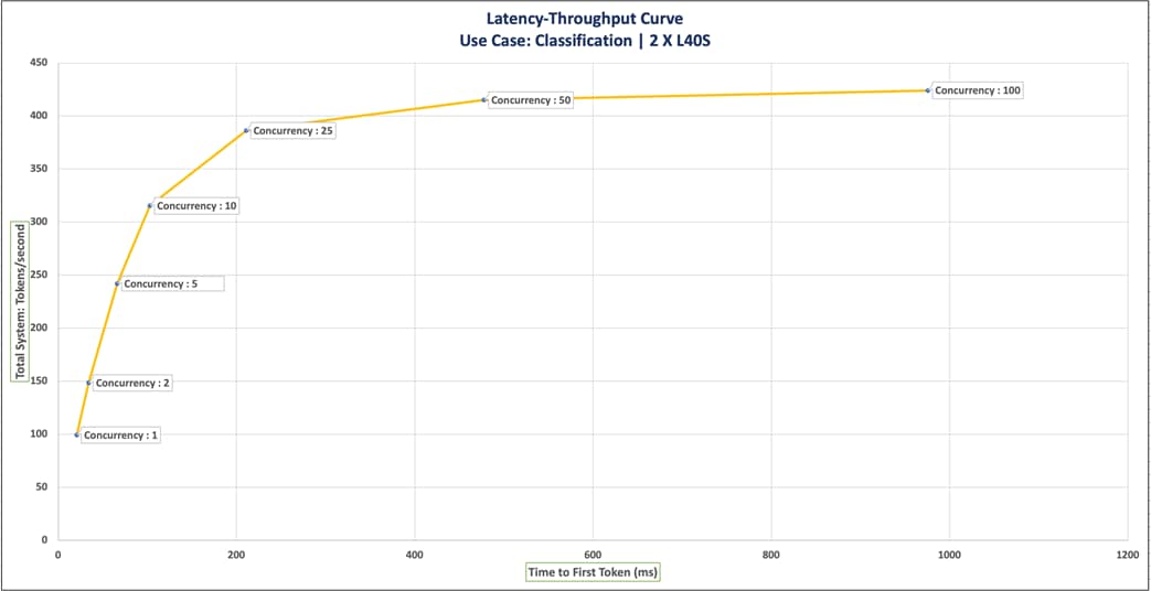
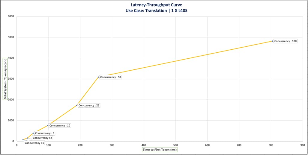
● Axes Definitions
◦ X-axis: Time to First Token (TTFT) - The duration a user waits before the model starts generating output.
◦ Y-axis: Total System Throughput - The total number of output tokens generated per second.
◦ Dots: Represent different concurrency levels.
Usage Guidelines
● Latency Budget Approach
Objective: Determine the highest achievable throughput within a specified latency limit.
Method: Identify the maximum acceptable TTFT on the X-axis, then find the corresponding Y value and concurrency level. This indicates the highest throughput achievable within the given latency constraint.
● Concurrency-Based Approach
Objective: Understand the latency and throughput for a specific concurrency level.
Method: Locate the desired concurrency level on the plot. The intersecting X and Y values represent the latency and throughput for that concurrency.
● Key Observations
The Latency-Throughput Curve for Classification plot highlights concurrency levels where latency increases significantly with minimal or no throughput gain. Concurrency = 50 is an example of such a point.
● Alternative Metrics
Similar plots can be generated using different metrics on the X-axis, such as ITL (Inference Time Latency), e2e_latency (End-to-End Latency), or TPS_per_user (Transactions Per Second per User). These plots help visualize the trade-offs between total system throughput and individual user latency.
Memory Calculations for LLM Inferencing
Total Memory required is the sum of model memory size and the KV cache.
Calculations for the required total memory are provided below:
Model Memory Size = Model Parameters * Precision
KV Cache Size = 2 x Batch Size x Context Size x Number of Layers x Model Dimensions x Precision
Total Memory Requirements (GB) = Model Memory Size (GB) + KV Cache Size (GB)
For some models, model dimension data might not be available. In that case, model dimension can be calculated as:
Model Dimensions = Attention Head Size X Number of Attention Heads
Model Parameters, Precision, Number of layers, Model Dimension are specific to models, and it can be found in the Model card for the model.
Context Size and batch size are input from users.
The following is an example memory calculation for Llama 2:

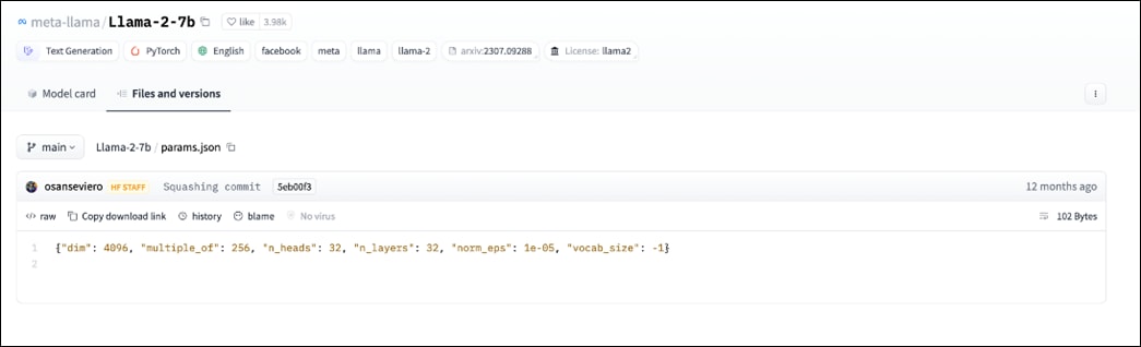
For the Llama 2 model:
Total model parameters: 6.74B Parameters.
Precision: FP16. (2 Bytes)
Number of layers: 32
Model Dimension: 4096
Therefore, the model memory is calculated as shown below:
Model Memory Size = Model Parameters * Precision
Model Memory Size for Llama 2 = 6,740,000,000 * 2 Bytes/Parameter
= 13,480,000,000 Bytes
= 13.48 Giga Bytes
Also, considering an example of maximum Input Tokens Length of 1024, Maximum Output Tokens Length of 1024, and the Batch size of 8, below are the calculations for KV Cache Size:
KV Cache Size = 2 x Batch Size x Context Size x Number of Layers x Model Dimensions x Precision
KV Cache Size = 2 x 8 x (1024+1024) x 32 x 4096 x 2 Bytes/Parameter
= 8,589,934,592 Bytes
= 8.59 Giga Bytes
Therefore, Llama2 with maximum Input Tokens Length of 1024, Maximum Output Tokens Length of 1024, and the Batch size of 8, the total memory required is shown below:
Total Memory Requirements (GB) = Model Memory Size (GB) + KV Cache Size (GB)
= 13.48 + 8.59 Giga Bytes
= 22.07 Giga Bytes
Performance Calculations
Note: The performance benchmark can be run on model.
Based on the performance requirement, number of users, number of input and output tokens, latency and throughput required, you can choose the appropriate Large Language Model, Inferencing backend, GPUs, and compute infrastructure.
Performance of the model depends on the prefill and decode phases. These two phases have different impacts on the performance of the LLM. While the prefill phase effectively saturates GPU compute at small batch sizes, the decode phase results in low compute utilization as it generates one token at a time per request.
The prefill phase is compute-bound, while the decode phase is memory-bound. So, the following factors need to be considered and measured:
● Prefill Latency
● Prefill Throughput
● Decode Total Latency
● Decode Token Latency
● Decode Throughput
The performance benchmark can be run with different sizes (1,2,4,8,10,25,250, 100 and so on). Also, separate tests can be run focused on performance comparison between 2 different models.
How RAG Works
Retrieval-Augmented Generation (RAG) is a technique used to enrich LLM outputs by using additional relevant information from an external knowledge base. This allows an LLM to generate responses based on context beyond the scope of its training data.
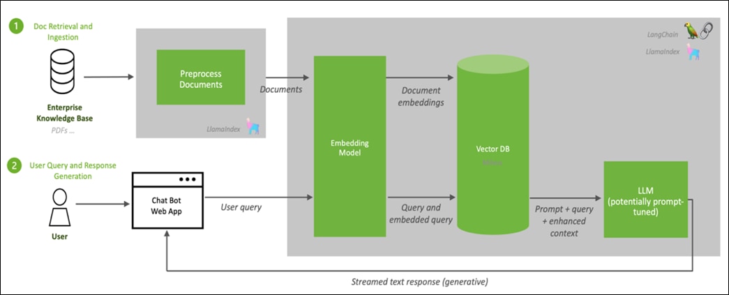
Why Evaluate RAG?
RAG enhances content generation by leveraging existing information effectively. It can amalgamate specific, relevant details from multiple sources to generate more accurate and relevant query results. This makes RAG potentially invaluable in various domains, including content creation, question & answer applications, and information synthesis. RAG does this by combining the strengths of retrieval, usually using dense vector search, and text generation, but to see what is and isn't working in your RAG system, to refine and optimize, you must evaluate it.
Note: Evaluation is essential to validate and make sure your application does what is expected.
Evaluation Process
Evaluating RAG goes through the following steps:
1. Choose Right Evaluation Framework.
2. Generate Synthetic Dataset.
3. Generate RAG Outputs for the Questions from Synthetic Dataset.
4. Evaluating Using the Generated Dataset.
5. Understanding The Metrics.
Choose the Right Evaluation Framework
RAG evaluation quantifies the accuracy of retrieval phrase by calculating metrics on the top results your system returns, enabling you to programmatically monitor pipeline’s precision, recall ability, and faithfulness to facts.

It is not only important to have good metrics, but that the ability to measure things separately.

To see where things are going well, can be improved, and where errors may originate, it's important to evaluate each component in isolation. The Figure 28 classifies the RAG’s components – along with what needs evaluation in each:
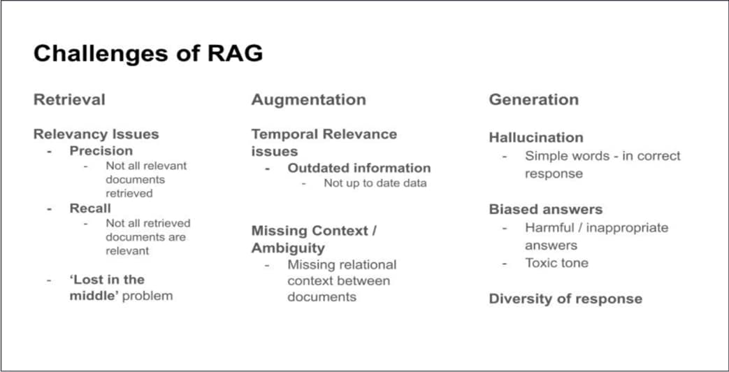
The Evaluation Framework is meant to ensure granular and thorough measurement, addressing the challenges faced in all three components.
To meet the evaluation challenges systematically, it’s a best practice to breakdown evaluation into different levels.
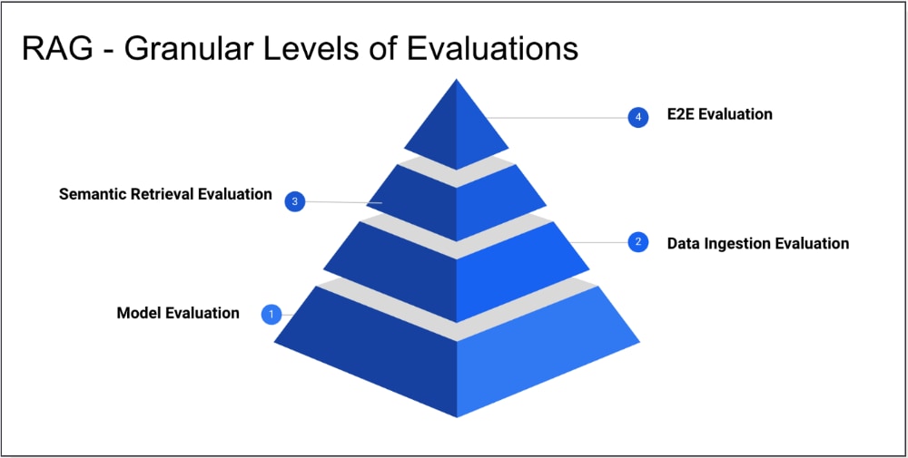
Embedding Model Evaluation
The Massive Text Embedding Benchmark (MTEB) leverages different public/private datasets to evaluate and report on the different capabilities of individual models. You can use the MTEB to evaluate any model in its list
The Model used in this deployment type is “snowflake-arctic-embed-I” and below is the model’s performance listed on leaderboard:
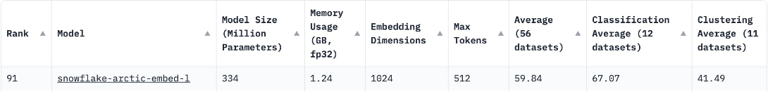
Data Ingestion Evaluation
After evaluating model’s performance using benchmarks, and (optionally) fine-tune it, then configure data ingestion into semantic retrieval store (vector store).
To evaluate data ingestion, observe and measure how changes in related variables affect ingestion outcomes:
● Chunk Size: The size of each data segment, which depends on the token limit of the embedding model. Chunk size substantially determines data granularity and the contextual understanding of the data, which impacts the precision, recall, and relevancy of results.
● Chunk Overlap: The extent to which data points of events are shared by adjacent data chunks. Overlap helps with retention of context information contained in chunks but should be paired with strategies like deduplication and content normalization to eradicate adverse effects (redundancy or inconsistency).
● Chunking/ Text Splitting Strategy: The process of data splitting and further treatment, based on both data type (for example, html, markdown, code, or pdf, and so on) and nuances of your use case.
Semantic Retrieval Evaluation
In this deployment, the Milvus Vector Database has been deployed, and milvus offers similarity metrics.
Similarity metrics are used to measure similarities among vectors. Choosing a good distance metric helps improve the classification and clustering performance significantly.
| Similarity Metrics |
Index Type |
|
● Euclidean distance (L2)
● Inner Product (IP)
|
● FLAT
● IVF_FLAT
● IVF_SQ8
● IVF_PQ
● HNSW
● IVF_HNSW
● RHNSW_FLAT
● RHNSW_SQ
● RHNSW_PQ
● ANNOY
|
Euclidean distance (L2)—essentially, Euclidean distance measures the length of a segment that connects 2 points.
The formula for Euclidean distance is as follows:

where a = (a1, a2,…, an) and b = (b1, b2,…, bn) are two points in n-dimensional Euclidean space
It’s the most used distance metric and is very useful when the data are continuous.
Inner Product (IP)—The IP distance between two embeddings is defined as follows:

Where A and B are embeddings, ||A|| and ||B|| are the norms of A and B.
IP is more useful if you are more interested in measuring the orientation but not the magnitude of the vectors.
If you use IP to calculate embeddings similarities, you must normalize your embeddings. After normalization, the inner product equals cosine similarity.
Suppose X’ is normalized from embedding X:

The correlation between the two embeddings is as follows:

End-to-End Evaluation
An end-to-end evaluation of a RAG application assesses the final outputs generated by LLMs in response to given inputs. It requires addressing issues discussed above related to data heterogeneity, domain specificity, and user query and preference diversity. It's impossible to devise a fixed metric or methodology that fits all domains and use cases.
E2E evaluation frameworks range from proprietary solutions to open-source tools. Selecting the right solution requires balancing considerations around ease of maintenance and operational burden, plus how well the metrics observed by the tool map to your Retrieval Augmented Generation pipeline’s use case.
Table 26. Recommended RAG Frameworks based on Use Case
| Use Case |
Framework |
Metrics Used |
Reasoning |
| Initial RAG Evaluations |
RAGAS |
Average Precision (AP), Faithfulness |
RAGAS is ideal for initial evaluations, especially in environments where reference data is scarce. It focuses on precision and how faithfully the response matches the provided context. |
| Dynamic, Continuous RAG Deployments |
ARES |
MRR, NDCG |
ARES uses synthetic data and LLM judges, which are suitable for environments needing continuous updates and training and focusing on response ranking and relevance. |
| Full System Traces, Including LLM’s and Vector Storage |
TraceLoop |
Informational Gain, Factual Consistency, Citation Accuracy |
TraceLoop is best suited for applications where tracing the flow and provenance of information used in the generated output is critical, such as academic research or journalism. |
| Realtime RAG Monitoring |
Arize |
Precision, Recall, F1 |
Arize excels in real-time performance monitoring, making it perfect for deployments where immediate feedback on RAG performance is essential |
| Enterprise Level RAG Applications |
Galileo |
Custom Metrics, Context Adherence |
Galileo provides advanced insights and metrics integration for complex applications, ensuring RAG’s adherence to context. |
| Optimizing RAG for Specific Domains |
TruLens |
Domain-Specific Accuracy, Precision |
TruLens is designed to optimize RAG systems within specific domains, by enhancing the accuracy and precision of domain-relevant responses |
Since a satisfactory LLM output depends entirely on the quality of the retriever and generator, RAG evaluation focuses on evaluating the retriever and generator in RAG pipeline separately. This allows for easier debugging and to pinpoint issues on a component level.
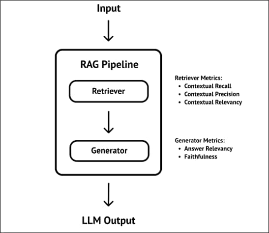
This document provides the steps necessary to run RAGAS Evaluation Framework. RAGAS is a framework that helps evaluate Retrieval Augmented Generation (RAG) Initial pipelines.
Generate Synthetic Dataset
To set up RAGAS evaluation Framework, apply ground truth concept. Some ground truth data - a golden set - provides a meaningful context for the metrics to evaluate our RAG pipeline's generated responses.
The first step in setting up RAGAS is creating an evaluation dataset, complete with questions, answers, and ground-truth data, which takes account of relevant context.
Procedure 1. Create an evaluation dataset
Step 1. Create LLM Prompt template:
LLM_PROMPT_TEMPLATE = (
"<s>[INST] <<SYS>>"
"{system_prompt}"
"<</SYS>>"
" "
"[The Start of the Reference Context]"
"{ctx_ref}"
"[The End of Reference Context][/INST]"
)
Step 2. Create the System template:
SYS_PROMPT = """
Given the context paragraph, create two very good question answer pairs.
Your output should be strictly in a json format of individual question answer pairs with keys from ["question","answer"].
Restrict the question to the context information provided.
"""
Step 3. Generate Synthetic Data:
def generate_synthetic_data(
dataset_folder_path,
qa_generation_file_path,
text_splitter_params={"chunk_size": 3000, "chunk_overlap": 100},
):
files=[dataset_folder_path]
llm = ChatNVIDIA(base_url="http://10.102.2.216:31641/v1", model="meta/llama3-8b-instruct",nvidia_api_key="not-used", max_tokens=1024)
json_data = []
i = 0
for pdf_file in files:
i += 1
try:
logger.info(f"{i}/{len(files)}")
# pdf_file = dataset_folder_path +'/'+ pdf_file
loader = PyPDFLoader(pdf_file)
data = loader.load()
text_splitter = RecursiveCharacterTextSplitter(**text_splitter_params)
all_splits = text_splitter.split_documents(data)
for split in all_splits:
context = LLM_PROMPT_TEMPLATE.format(
system_prompt=SYS_PROMPT,
ctx_ref=split.page_content)
try:
answer = llm.invoke(context).content
question_pattern = r'"question":\s*"([^"]*)"'
answer_pattern = r'"answer":\s*"([^"]*)"'
question_match = re.findall(question_pattern, answer)
answer_match = re.findall(answer_pattern, answer)
if(len(question_match)==len(answer_match)):
for j, _ in enumerate(question_match):
my_data = {
'question': question_match[j],
'ground_truth_answer': answer_match[j],
'ground_truth_context': split.page_content,
'document': pdf_file,
}
json_data.append(my_data)
except Exception as e:
logger.info(
f"\n PDF: {pdf_file} \n \t Context: {context} \n Exception Occured: {e}"
)
except Exception as e:
logger.info(f"\n PDF: {pdf_file} \n Exception Occured: {e}")
with open(qa_generation_file_path, "w", encoding="utf-8") as f:
json.dump(json_data, f)
Step 4. Call this function with path to the document and file name for q&a:
generate_synthetic_data('/home/admin/RAG/flashstack_ai_generative_ocp_m7.pdf','/home/admin/RAG/flashstack_qa_generation.json')
This creates a JSON file called “flashstack_qa_generation.json”
Procedure 2. Generate RAG Outputs for the Questions from Synthetic Dataset
Step 1. Load the JSON file and iterate through each question, retrieve context from vector store and ask LLM to generate the response:
url_upload = f"http://10.102.2.216:31935/documents"
url_generate = f"http://10.102.2.216:31935/generate"
url_doc_search = f"http://10.102.2.216:31935/search"
f = open('/home/admin/RAG/flashstack_qa_generation.json')
data = json.load(f)
generate_api_params={"use_knowledge_base": True, "temperature":0.2,"top_p":0.7,"max_tokens": 256}
document_search_api_params={"num_docs": 1}
new_data=[]
for entry in data:
entry_generate = {
"messages":[
{
"role":"user",
"content":entry["question"]
}
],
"use_knowledge_base": generate_api_params["use_knowledge_base"],
"temperature": generate_api_params["temperature"],
"top_p": generate_api_params["top_p"],
"max_tokens": generate_api_params["max_tokens"],
"stop":[
"string"
]
}
entry["answer"] = ""
try:
with requests.post(url_generate, stream=True, json=entry_generate) as r:
for chunk in r.iter_lines():
raw_resp = chunk.decode("UTF-8")
if not raw_resp:
continue
resp_dict = None
try:
print(raw_resp)
resp_dict = json.loads(raw_resp[6:])
resp_choices = resp_dict.get("choices", [])
if len(resp_choices):
resp_str = resp_choices[0].get("message", {}).get("content", "")
entry["answer"] += resp_str
except Exception as e:
print(f"Exception Occured: {e}")
except Exception as e:
print(f"Exception Occured: {e}")
entry["answer"] = "Answer couldn't be generated."
print(entry["answer"])
entry_doc_search = {
"query": entry["question"],
"top_k": document_search_api_params["num_docs"]
}
response = requests.post(url_doc_search, json=entry_doc_search).json()
context_list =typing.cast(typing.List[typing.Dict[str, typing.Union[str, float]]], response)
contexts = [context.get("content") for context in context_list['chunks']]
try:
entry["contexts"] = [contexts[0]]
except Exception as e:
print(f"Exception Occured: {e}")
entry["contexts"] = ""
new_data.append(entry)
Step 2. Once the new list of objects is created, store them on the file system as shown below:
with open('/home/admin/RAG/flashstack_eval.json', 'w') as f:
json.dump(data, f)
This creates a JSON file called “flashstack_eval.json”
Procedure 3. Evaluate using the Generated Dataset
Step 1. Create the Prompt Template:
LLAMA_PROMPT_TEMPLATE = (
"<s>[INST] <<SYS>>"
"{system_prompt}"
"<</SYS>>"
""
"Example 1:"
"[Question]"
"When did Queen Elizabeth II die?"
"[The Start of the Reference Context]"
"""On 8 September 2022, Buckingham Palace released a statement which read: "Following further evaluation this morning, the Queen's doctors are concerned for Her Majesty's health and have recommended she remain under medical supervision. The Queen remains comfortable and at Balmoral."[257][258] Her immediate family rushed to Balmoral to be by her side.[259][260] She died peacefully at 15:10 BST at the age of 96, with two of her children, Charles and Anne, by her side;[261][262] Charles immediately succeeded as monarch. Her death was announced to the public at 18:30,[263][264] setting in motion Operation London Bridge and, because she died in Scotland, Operation Unicorn.[265][266] Elizabeth was the first monarch to die in Scotland since James V in 1542.[267] Her death certificate recorded her cause of death as old age"""
"[The End of Reference Context]"
"[The Start of the Reference Answer]"
"Queen Elizabeth II died on September 8, 2022."
"[The End of Reference Answer]"
"[The Start of the Assistant's Answer]"
"She died on September 8, 2022"
"[The End of Assistant's Answer]"
'"Rating": 5, "Explanation": "The answer is helpful, relevant, accurate, and concise. It matches the information provided in the reference context and answer."'
""
"Example 2:"
"[Question]"
"When did Queen Elizabeth II die?"
"[The Start of the Reference Context]"
"""On 8 September 2022, Buckingham Palace released a statement which read: "Following further evaluation this morning, the Queen's doctors are concerned for Her Majesty's health and have recommended she remain under medical supervision. The Queen remains comfortable and at Balmoral."[257][258] Her immediate family rushed to Balmoral to be by her side.[259][260] She died peacefully at 15:10 BST at the age of 96, with two of her children, Charles and Anne, by her side;[261][262] Charles immediately succeeded as monarch. Her death was announced to the public at 18:30,[263][264] setting in motion Operation London Bridge and, because she died in Scotland, Operation Unicorn.[265][266] Elizabeth was the first monarch to die in Scotland since James V in 1542.[267] Her death certificate recorded her cause of death as old age"""
"[The End of Reference Context]"
"[The Start of the Reference Answer]"
"Queen Elizabeth II died on September 8, 2022."
"[The End of Reference Answer]"
"[The Start of the Assistant's Answer]"
"Queen Elizabeth II was the longest reigning monarch of the United Kingdom and the Commonwealth."
"[The End of Assistant's Answer]"
'"Rating": 1, "Explanation": "The answer is not helpful or relevant. It does not answer the question and instead goes off topic."'
""
"Follow the exact same format as above. Put Rating first and Explanation second. Rating must be between 1 and 5. What is the rating and explanation for the following assistant's answer"
"Rating and Explanation should be in JSON format"
"[Question]"
"{question}"
"[The Start of the Reference Context]"
"{ctx_ref}"
"[The End of Reference Context]"
"[The Start of the Reference Answer]"
"{answer_ref}"
"[The End of Reference Answer]"
"[The Start of the Assistant's Answer]"
"{answer}"
"[The End of Assistant's Answer][/INST]"
)
Step 2. Create System Prompt:
SYS_PROMPT = """
You are an impartial judge that evaluates the quality of an assistant's answer to the question provided.
You evaluation takes into account helpfullness, relevancy, accuracy, and level of detail of the answer.
You must use both the reference context and reference answer to guide your evaluation.
"""
The performance of individual components within the LLM and RAG pipeline has a significant impact on the overall experience. Ragas offers metrics tailored for evaluating each component of RAG pipeline in isolation.
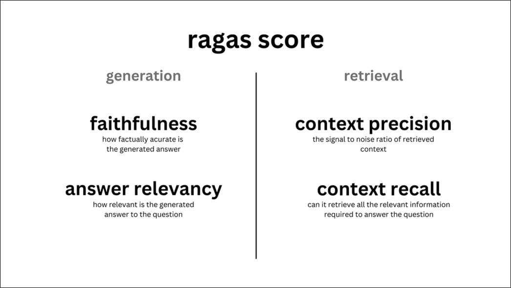
Step 3. Create a Function to choose the metric types:
def calculate_ragas_score(row):
values = row[['faithfulness', 'context_relevancy', 'answer_relevancy','context_recall']].values
return statistics.harmonic_mean(values)
Step 4. Create a Function to run RAGAS Evaluation from the evaluation json dataset:
def eval_ragas(ev_file_path, ev_result_path,llm_model='ai-mixtral-8x7b-instruct'):
"""
This function evaluates a language model's performance using a dataset and metrics.
It sets the NVAPI_KEY, initializes a ChatNVIDIA model and LangchainLLM object, loads the
evaluation dataset, prepares data samples, creates a Dataset object, sets the language model
for each metric, and evaluates the model with the specified metrics, printing the results.
"""
llm = ChatNVIDIA(base_url="http://10.102.2.216:31641/v1", model="meta/llama3-8b-instruct",nvidia_api_key="not-used", max_tokens=1024)
nvpl_llm = LangchainLLMWrapper(langchain_llm=llm)
model = "NV-Embed-QA"
url="http://10.102.2.216:32128/v1/embeddings"
batch_size=32
embeddings = NeMoEmbeddings(
batch_size=batch_size, model=model, api_endpoint_url=url
)
nvpl_embeddings = LangchainEmbeddingsWrapper(embeddings)
try:
with open(ev_file_path, "r", encoding="utf-8") as file:
json_data = json.load(file)
except Exception as e:
logger.info(f"Error Occured while loading file : {e}")
eval_questions = []
eval_answers = []
ground_truth = []
vdb_contexts = []
for entry in json_data:
eval_questions.append(entry["question"])
eval_answers.append(entry["answer"])
vdb_contexts.append(entry['contexts'])
ground_truth.append(entry["ground_truth_answer"])
data_samples = {
'question': eval_questions,
'answer': eval_answers,
'contexts': vdb_contexts,
'ground_truth': ground_truth,
}
# print(data_samples)
dataset = Dataset.from_dict(data_samples)
print(dataset)
result = evaluate(
dataset,
llm=llm,
embeddings=nvpl_embeddings,
metrics=[
answer_similarity,
faithfulness,
context_precision,
context_relevancy,
answer_relevancy,
context_recall
],
)
df = result.to_pandas()
df['ragas_score']=df.apply(calculate_ragas_score,axis=1)
df.to_parquet(ev_result_path+'.parquet')
result['ragas_score']= statistics.harmonic_mean([result['faithfulness'], result['context_relevancy'], result['answer_relevancy'], result['context_recall']])
with open(ev_result_path+'.json', "w", encoding="utf-8") as json_file:
json.dump(result, json_file, indent=2)
The following are the results:
eval_ragas('/home/admin/RAG/flashstack_eval.json','/home/admin/RAG/results/flashstack_evaluator')
{
"answer_similarity": 0.5262431058841802,
"faithfulness": 0.7325238095238095,
"context_precision": 0.9799999999019999,
"context_relevancy": 0.2949610417961811,
"answer_relevancy": 0.5797973179159244,
"context_recall": 0.8744285714285713,
"ragas_score": 0.5246750611338722
}
Understanding the Metrics
● Answer Similarity
The concept of Answer Semantic Similarity pertains to the assessment of the semantic resemblance between the generated answer and the ground truth. This evaluation is based on the ground truth and the answer, with values falling within the range of 0 to 1. A higher score signifies a better alignment between the generated answer and the ground truth.
Measuring the semantic similarity between answers can offer valuable insights into the quality of the generated response. This evaluation utilizes a cross-encoder model to calculate the semantic similarity score.
● Faithfulness
This measures the factual consistency of the generated answer against the given context. It is calculated from answer and retrieved context. The answer is scaled to (0,1) range. Higher the better.
The generated answer is regarded as faithful if all the claims made in the answer can be inferred from the given context. To calculate this, a set of claims from the generated answer is first identified. Each of these claims is cross-checked with the given context to determine if it can be inferred from the context. The faithfulness score is determined by:

● Context Precision
Context Precision is a metric that evaluates whether all the ground-truth relevant items present in the contexts are ranked higher or not. Ideally all the relevant chunks must appear at the top ranks. This metric is computed using the question, ground_truth and the contexts, with values ranging between 0 and 1, where higher scores indicate better precision.

Where K is the total number of chunks in contexts and vk∈ {0,1} is the relevance indicator at rank k.
● Context Relevancy
This metric gauge the relevancy of the retrieved context, calculated based on both the question and contexts. The values fall within the range of (0, 1), with higher values indicating better relevancy.
Ideally, the retrieved context should exclusively contain essential information to address the provided query. To compute this, we initially estimate the value of |S| by identifying sentences within the retrieved context that are relevant for answering the given question. The final score is determined by the following formula:

● Answer Relevancy
The evaluation metric, Answer Relevancy, focuses on assessing how pertinent the generated answer is to the given prompt. A lower score is assigned to answers that are incomplete or contain redundant information and higher scores indicate better relevancy. This metric is computed using the question, the context, and the answer.
The Answer Relevancy is defined as the mean cosine similarity of the original question to a number of artificial questions, which were generated (reverse engineered) based on the answer:

Where:
● Egi is the embedding of the generated question i.
● Eo is the embedding of the original question.
● N is the number of generated questions, which is 3 default.
Note: Even though in practice the score will range between 0 and 1 most of the time, this is not mathematically guaranteed, due to the nature of the cosine similarity ranging from -1 to 1.
● Context Recall
Context recall measures the extent to which the retrieved context aligns with the annotated answer, treated as the ground truth. It is computed using question, ground truth and the retrieved context, and the values range between 0 and 1, with higher values indicating better performance. To estimate context recall from the ground truth answer, each claim in the ground truth answer is analyzed to determine whether it can be attributed to the retrieved context or not. In an ideal scenario, all claims in the ground truth answer should be attributable to the retrieved context. A reference free version of this is available as context_utilization.
The formula for calculating context recall is as follows:

● RAGAS Score
This metric provides a measure of how well the summary captures the important information from the contexts. The intuition behind this metric is that a good summary shall contain all the important information present in the context (or text).
First extract a set of important key phrases from the context. These key phrases are then used to generate a set of questions. The answers to these questions are always yes (1) for the context. Ask these questions to the summary and calculate the summarization score as the ratio of correctly answered questions to the total number of questions.
Compute the question-answer score using the answers, which is a list of 1s and 0s. The question-answer score is then calculated as the ratio of correctly answered questions (answer = 1) to the total number of questions.

Milvus Benchmarking with VectorDBBench
Today, the growth of unstructured data and the rise of AI and LLMs have highlighted vector databases as a crucial component of the infrastructure. As the focus shifts to these tools, enterprises need to assess and select the right one for their business. Vector databases manage unstructured data like images, video, text and so on, using vector embeddings. Vector databases specialize in semantic similarity searches using a machine-learning technique called Approximate Nearest Neighbor (ANN). Vector databases are the vector store for RAG applications.
Milvus is a high-performance, highly scalable vector database that runs efficiently across a wide range of environments. Unstructured data varies in format and carries rich underlying semantics, making it challenging to analyze. To manage this complexity, embeddings are used to convert unstructured data into numerical vectors that capture its essential characteristics. These vectors are then stored in a vector database, enabling fast and scalable searches and analytics. Milvus offers robust data modeling capabilities, enabling you to organize your unstructured or multi-modal data into structured collections. Milvus allocates over 80% of its computing resources to its vector databases and search engine. Given the computational demands of high-performance computing, GPUs emerge as a pivotal element of vector database platform, especially within the vector search domain.
NVIDIA’s latest innovation, the GPU-based graph index CAGRA (CUDA ANNs GRAph-based), represents a significant milestone. With NVIDIA’s assistance, Milvus integrated support for CAGRA in its 2.4 version, marking a significant stride toward overcoming the obstacles of efficient GPU implementation in vector search.
The decision to leverage GPU indexes was primarily motivated by performance considerations. We undertook a comprehensive evaluation of Milvus’ performance utilizing the VectorDBBench tool, focusing on CAGRA index and observing key evaluation metrics like QPS (Queries Per Second), latency, and recall.
VectorDBBench is the best performing and cost-effective comparison open-source tool, and it offers more than just benchmark results for popular vector databases and cloud services.
Query Performance Metrics
Assessing the query performance of vector databases typically involves three key metrics: latency, queries per second (QPS), and recall rate.
Latency testing measures the time taken for a single query under serial testing conditions. P99 latency is a commonly used metric representing the duration within which 99% of queries are completed. It offers a more nuanced perspective than average latency and aligns closely with user experience.
Note: While latency testing is straightforward, it's heavily influenced by network conditions, especially for cloud products.
QPS refers to a database's query capability under high concurrency. It is achieved by simultaneously sending multiple requests from the test client to maximize database CPU/ GPU utilization and observe throughput. Unlike latency, QPS is less susceptible to network fluctuations, providing a comprehensive evaluation of a vector database's real-world performance.
Recall is the proportion of the ground truth documents that are represented in the retrieved chunks. This is a measure of the completeness of the results.
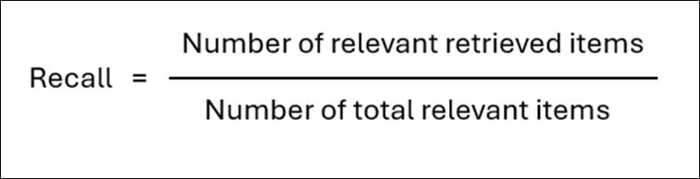
High recall ensures that the LLM is comprehensive in its responses, capturing all the relevant information necessary for the task.
Procedure 1. Milvus Distributed deployment with FlashBlade//S
Vector database benchmarking is executed with Milvus Distributed vector database with NVIDIA L40S GPUs. For detailed steps on deploying Distributed Milvus vector database, go to section Vector Database.
For detailed information, click the following links:
● https://milvus.io/docs/install_cluster-helm-gpu.md
● https://github.com/milvus-io/milvus
VectorDBBench
VectorDBBench is an open-source benchmarking tool designed for high-performance data storage and retrieval systems. This tool allows users to test and compare different vector database systems' performance to determine their specific use case's most suitable database system. Using VectorDBBench, users can make informed decisions based on the actual vector database performance of the systems they are evaluating.
VectorDBBench is written in Python and licensed under the MIT open-source license, The tool is actively maintained by a community of developers committed to improving its features and performance.
Procedure 1. Install and run the VectorDBBench tool
Step 1. Prerequisite:
Python >= 3.11
Step 2. Create a virtual python environment “milvus” and activate it:
python -m venv milvus
source milvus/bin/activate
cd milvus
Step 3. Install vectordb-bench:
pip install vectordb-bench==0.0.22
Step 4. Run vectordb-bench:
python -m vectordb_bench
OR
init_bench
After completion, the tool is up and running and can access the streamlit web application using the network URL.
Step 5. After completion of the benchmark testing with vectordb-bench tool, to come out of the python virtual environment, run the following script:
deactivate
For more information, see: https://github.com/zilliztech/VectorDBBench
Procedure 2. Run the Test
Step 1. Select the database(s). There are various options available for vector databases like Milvus, Pinecone, PgVector, and so on.
Note: In our tests, we used Milvus.
Step 2. Provide the required configuration information for the selected database:
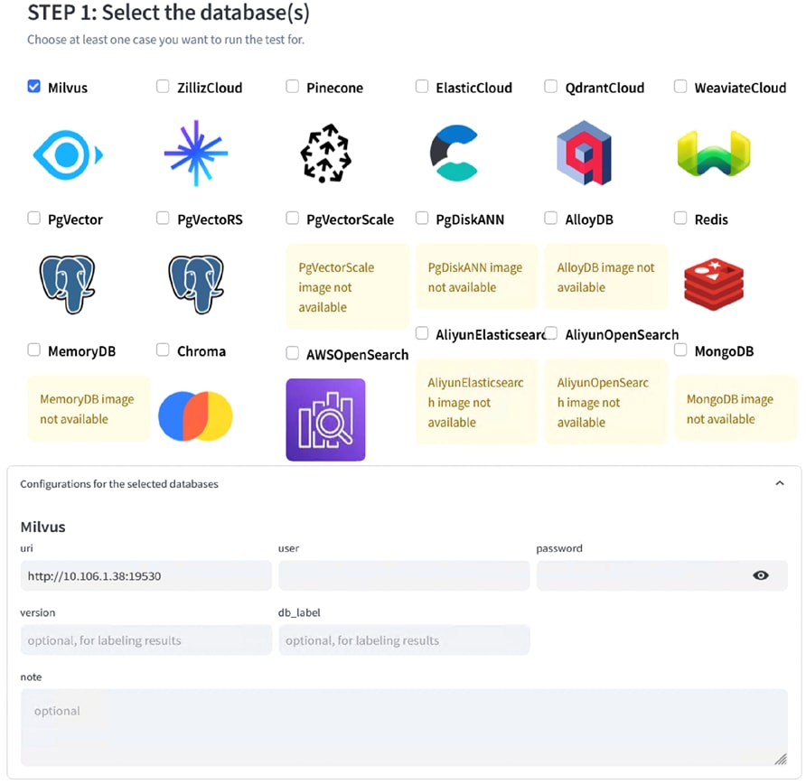
Step 3. Select the test case to run the benchmarking test.
Note: We ran a Search Performance Test case with a medium dataset (Cohere 1M vectors, 768 dimensions)
Step 4. Select the index type. You can select the index type depending upon their deployment characteristics and datasets. Some of the options provided by vectordbbench are DISKANN, HNSW, GPU_IVF_FLAT, GPU_IVF_PQ and so on. There is a flexibility provided to change the test parameters pertaining to a particular index type.
Note: We used GPU_CAGRA and HSNW indexes with default parameters for running the tests.
● HSNW index type (CPU based):
The HNSW index is a graph-based indexing algorithm that can improve performance when searching for high-dimensional floating vectors. It offers excellent search accuracy and low latency but with the tradeoff of long index build time and it requires high memory overhead to maintain its hierarchical graph structure. For more details on this index type, refer: https://milvus.io/docs/hnsw.md
● GPU_CAGRA Index Type (GPU-based)
GPU_CAGRA is a graph-based index optimized for GPUs. Using inference-grade GPUs to run the Milvus GPU version can be more cost-effective compared to using expensive training-grade GPUs.
Note: For more information about index building and search parameters, go to: https://milvus.io/docs/gpu_index.md.
Note: For detailed information about the integration of milvus with CAGRA, go to: https://zilliz.com/blog/Milvus-introduces-GPU-index-CAGRA
Step 5. You can provide your custom task label or go by default as provided by the tool.
Benchmarking Test Details
In this solution, we executed Search Performance test of Milvus vectorstore DB with Cohere 1M dataset size and 768 dimensions and varied the batch size for the ML model. Latencyp99, recall, load-duration, and QPS (Queries Per Second) are the few KPIs used to validate the test results. These tests were executed for both HSNW and GPU_CAGRA index types.
To update the batch size between test iterations, update the NUM_PER_BATCH variable in the __init__.py file which is stored under python3.12/site-packages/vectordb_bench/ directory.
Note: We used batch sizes of 1, 10, 50, and 100 in the test iterations.
Note: The dataset gets downloaded on the client machine where vectordb_bench is running. Therefore, make sure there is sufficient disk space on the system.
Since these tests are executed with HSNW (CPU based) and GPU_CAGRA (GPU based) indexes, CPU utilization for HSNW and GPU utilization for GPU_CAGRA index were captured during the tests.
Test Results
This chapter contains the following:
● Test Results for HSNW Index Search Performance
● Test Results for GPU_CAGRA Index Search Performance
While running the test, we noticed that the CPU and GPU were being utilized during various stages of the test execution like data ingestion, query execution , and so on. The CPU and GPU utilizations are captured during Search Performance test execution with linux top and nvidia-smi tool.
Test Results for HSNW Index Search Performance
The following table lists the performance metrics for various batch sizes with Search Performance test executed with HSNW index type.
| Batch size |
Recall |
serial_latency_p99 (ms) |
QPS (Query per second) |
| 1 |
0.9767 |
2.9 |
5082 |
| 10 |
0.9704 |
2.9 |
6003 |
| 50 |
0.9704 |
2.9 |
6144 |
| 100 |
0.9704 |
2.9 |
6527 |
The following screenshot shows the CPU utilization by the query node during the Search Performance test execution. Milvus query node has consumed all the compute resources available on the worker node.
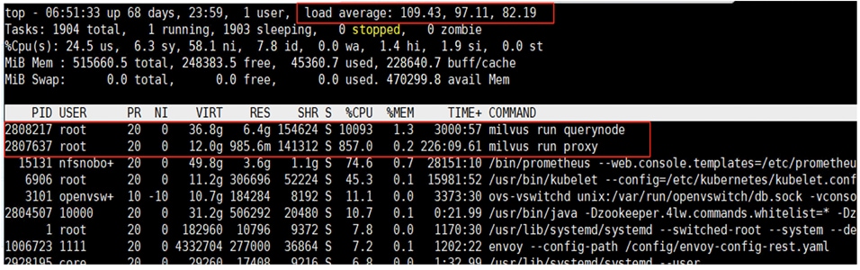
The HSNW index Search Performance numbers would vary and depend on the resources available on the underlying worker node where the query node is hosted.
Test Results for GPU_CAGRA Index Search Performance
The following table lists the performance metrics for various batch sizes with Search Performance test executed with GPU_CAGRA index type with one NVIDIA L40S GPU assigned to the milvus query node.
| Batch size |
Recall |
serial_latency_p99 (ms) |
QPS (Query per second) |
| 1 |
0.960 |
2.4 |
13229 |
| 10 |
0.9589 |
2.4 |
13250 |
| 50 |
0.9598 |
2.4 |
13276 |
| 100 |
0.9592 |
2.5 |
13291 |
The following screenshot shows the GPU utilization by the query node during the Search Performance test execution.
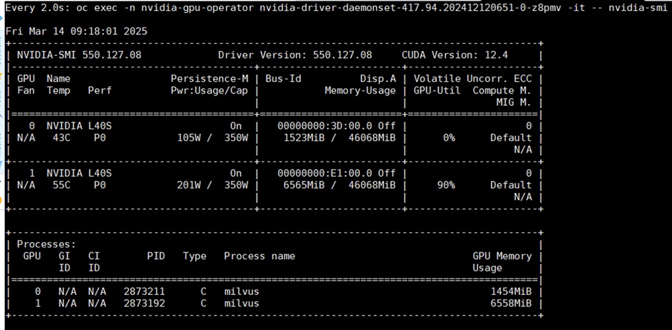
From these results, we can infer that as the batch size increases, the Multi Modal RAG performs better, that is validated by the trend in the output KPIs with Milvus vector store using VectorDBBench tool.
Note: Our test results are in agreement with the observations made by Zilliz as explained here: https://zilliz.com/blog/Milvus-introduces-GPU-index-CAGRA
QPS of GPU_CAGRA index is more than two times as that of HSNW index type. As explained earlier, the performance differences would vary depending on the type of GPU and CPUs used on the worker node.
The benchmark results underscore the substantial performance benefits of adopting GPU-accelerated indexes like CAGRA in Milvus. Not only does it excel in accelerating search tasks across batch sizes, but it also significantly enhances index construction speed, affirming the value of GPUs in optimizing vector database performance.
Conclusion
This Cisco Validated Design presents a robust and meticulously tested solution for deploying enterprise-grade Retrieval Augmented Generation (RAG) pipelines. By synergistically integrating the high-performance Cisco UCS X-Series based FlashStack infrastructure with the advanced capabilities of NVIDIA AI Enterprise software, including the RAG Blueprint and NVIDIA Inference Microservices (NIM), this architecture provides a streamlined path for leveraging generative AI with proprietary data.
The infrastructure is designed using the Cisco UCS X-Series modular platform based FlashStack Datacenter, managed through Cisco Intersight. Deployment involves Red Hat OpenShift Container Platform clusters running on Cisco UCS X210c M7 bare metal compute nodes equipped with NVIDIA GPUs. The NVIDIA AI Enterprise software powers the inferencing workflow, while Portworx Enterprise Storage, backed by Pure Storage FlashArray and FlashBlade, ensures cloud-native storage for model repositories and other services.
Automation facilitated by Red Hat Ansible, provides Infrastructure as Code (IaC) for accelerating deployments.
The FlashStack solution is a validated approach for deploying Cisco and Pure Storage technologies in an enterprise data center. This release of the FlashStack VSI solution brings the following capabilities:
● Fourth generation Intel Xeon Scalable processors with Cisco UCS X210 M7, C220 M7 and C240 M7 servers, enabling up to 60 cores per processor and 8TB of DDR-4800 DIMMs.
● Sustainability monitoring and optimizations to meet Enterprise ESG targets that include power usage monitoring features across all layers of the stack and utilizing the Cisco UCS X-Series advanced power and cooling policies.
● Pure Storage FlashArray Unified Block and File consisting of FC-SCSI, FC-NVMe, iSCSI, NVMe-TCP, NVMe-RoCEv2 as well as NFS and SMB storage.
● Pure Storage FlashBlade//S, a high-performance consolidated storage platform for both file (with native SMB and NFS support) and object (S3) workloads, delivering a simplified experience for infrastructure and data management.
● Red Hat Openshift innovations.
● Cisco Intersight continues to deliver features that simplify enterprise IT operations, with services and workflows that provide complete visibility and operations across all elements of FlashStack datacenter. Also, Cisco Intersight integration with VMware vCenter and Pure Storage FlashArray extends these capabilities and enable workload optimization to all layers of the FlashStack infrastructure.
Ultimately, this validated solution stands as a foundational reference architecture, significantly mitigating the complexities and risks associated with deploying sophisticated RAG workloads. It empowers enterprises to confidently build, manage, and scale secure, high-throughput private RAG applications, accelerating time-to-value for critical AI initiatives.
About the Authors
Paniraja Koppa, Technical Marketing Engineer, Cisco Systems, Inc.
Paniraja Koppa is a member of the Cisco Unified Computing System (Cisco UCS) solutions team. He has over 15 years of experience designing, implementing, and operating solutions in the data center. In his current role, he works on design and development, best practices, optimization, automation and technical content creation of compute and hybrid cloud solutions. He also worked as technical consulting engineer in the data center virtualization space. Paniraja holds a master’s degree in computer science. He has presented several papers at international conferences and speaker at events like Cisco Live US and Europe, Open Infrastructure Summit, and other partner events. Paniraja’s current focus is on Generative AI solutions.
Gopu Narasimha Reddy, Technical Marketing Engineer, Cisco Systems, Inc.
Gopu Narasimha Reddy is a Technical Marketing engineer with the UCS Solutions team at Cisco. He is currently focused on validating and developing Cisco UCS infrastructure solutions for enterprise workloads with different operating environments including Windows, VMware, Linux, and Kubernetes. Gopu is also involved in publishing database benchmarks on Cisco UCS servers. His areas of interest include building and validating reference architectures, and development of sizing tools in addition to assisting customers in database deployments.
Mahesh Pabba, Customer Delivery Architect, Cisco Systems, Inc.
Mahesh Pabba is a seasoned technology professional with vast experience in the IT industry. With a strong foundation in enterprise applications, he has successfully navigated various domains, excelling in automation and development using cutting-edge technologies. As a skilled Solution Architect, he has designed and implemented numerous innovative solutions throughout his career. Additionally, he possesses expertise in artificial intelligence, specializing in training, inferencing, and deploying AI solutions on Cisco hardware, encompassing compute, network, and storage environments. His unique blend of technical acumen and solution-oriented approach positions him as a valuable contributor to any AI design initiative.
Hang Yu, NVIDIA
Hang Yu is a Solutions Architect with expertise in AI/ML development and production. He focuses on the full-stack AI software, building and deploying enterprise-grade AI solutions, leading projects from initial design to production deployment. He has been working closely with Cisco on enabling this validated design.
Acknowledgements
For their support and contribution to the design, validation, and creation of this Cisco Validated Design, the authors would like to thank:
● Chris O’Brien, Senior Director, Technical Marketing, Cisco Systems, Inc.
● Umar Ali, Business Product Manager, Cisco Systems, Inc.
● Nitin Garg, Technical Marketing Engineering Technical Leader, Cisco Systems, Inc.
● Meenakshi Kaushik, NVIDIA
● Ruchika Kharwar, NVIDIA
● Sumit Bhattacharya, NVIDIA
● Nikhil Kulkarni, NVIDIA
● Nikita Jain, NVIDIA
● Anurag Guda, Technical Marketing Engineer, NVIDIA
● Craig Waters, Solutions Director, Pure Storage, Inc.
● Simranjit Singh, Solutions Architect, Pure Storage, Inc.
● Robert Alvarez, AI Solutions Architect, Pure Storage, Inc.
● Unnikrishnan R, Senior Solutions Architect, Pure Storage, Inc.
This appendix contains the following
● Appendix A – References used in this guide
Appendix A – References used in this guide
Compute
Cisco Intersight: https://www.intersight.com
Cisco Intersight Managed Mode: https://www.cisco.com/c/en/us/td/docs/unified_computing/Intersight/b_Intersight_Managed_Mode_Configuration_Guide.html
Cisco Unified Computing System X-Series Modular System: https://www.cisco.com/go/ucsx
Cisco UCS 6536 Fabric Interconnect Data Sheet: https://www.cisco.com/c/en/us/products/collateral/servers-unified-computing/ucs6536-fabric-interconnect-ds.html
AI-ready infrastructure - Cisco Validated Design Zone: https://www.cisco.com/c/en/us/solutions/design-zone/ai-ready-infrastructure.html
Cisco AI native infrastructure for Data Center: https://www.cisco.com/site/us/en/solutions/artificial-intelligence/infrastructure/index.html
Cisco Unified Compute System automation repositories for Cisco Validate Designs (CVD) and white papers: https://github.com/ucs-compute-solutions
Network
Cisco Nexus 9300-GX Series Switches: https://www.cisco.com/c/en/us/products/collateral/switches/nexus-9000-series-switches/nexus-9300-gx-series-switches-ds.html
Pure Storage
Pure Storage FlashArray//XL: https://www.purestorage.com/products/unified-block-file-storage/flasharray-xl.html
Pure Storage FlashBlade//S: https://www.purestorage.com/products/unstructured-data-storage/flashblade-s.html
Portworx by Pure Storage: https://docs.portworx.com/
FlashStack
FlashStack Design Guides: https://www.cisco.com/c/en/us/solutions/design-zone/data-center-design-guides/data-center-design-guides-all.html#FlashStack
FlashStack with Red Hat OCP and Virtualization platform CVD (Base CVD): https://www.cisco.com/c/en/us/td/docs/unified_computing/ucs/UCS_CVDs/flashstack_ocp_baremetal_imm.html
Red Hat OpenShift
Documentation: https://docs.openshift.com/
Red Hat OpenShift Container Platform: https://www.redhat.com/en/technologies/cloud-computing/openshift/container-platform
Red Hat Hybrid Cloud Console: https://cloud.redhat.com/
NVIDIA Enterprise
GitHub page for NVIDIA Blueprints: https://github.com/NVIDIA-AI-Blueprints
NVIDIA NIM Operator: https://docs.nvidia.com/nim-operator/latest/index.html
NVIDIA NIM Catalog: https://catalog.ngc.nvidia.com/
Interoperability Matrix
Cisco UCS Hardware Compatibility Matrix: https://ucshcltool.cloudapps.cisco.com/public/
Pure Storage FlashStack Compatibility Matrix. Note, this interoperability list will require a support login from Pure: https://support.purestorage.com/FlashStack/Product_Information/FlashStack_Compatibility_Matrix
Feedback
For comments and suggestions about this guide and related guides, join the discussion on Cisco Community here: https://cs.co/en-cvds.
CVD Program
ALL DESIGNS, SPECIFICATIONS, STATEMENTS, INFORMATION, AND RECOMMENDATIONS (COLLECTIVELY, "DESIGNS") IN THIS MANUAL ARE PRESENTED "AS IS," WITH ALL FAULTS. CISCO AND ITS SUPPLIERS DISCLAIM ALL WARRANTIES, INCLUDING, WITHOUT LIMITATION, THE WARRANTY OF MERCHANTABILITY, FITNESS FOR A PARTICULAR PURPOSE AND NONINFRINGEMENT OR ARISING FROM A COURSE OF DEALING, USAGE, OR TRADE PRACTICE. IN NO EVENT SHALL CISCO OR ITS SUPPLIERS BE LIABLE FOR ANY INDIRECT, SPECIAL, CONSEQUENTIAL, OR INCIDENTAL DAMAGES, INCLUDING, WITHOUT LIMITATION, LOST PROFITS OR LOSS OR DAMAGE TO DATA ARISING OUT OF THE USE OR INABILITY TO USE THE DESIGNS, EVEN IF CISCO OR ITS SUPPLIERS HAVE BEEN ADVISED OF THE POSSIBILITY OF SUCH DAMAGES.
THE DESIGNS ARE SUBJECT TO CHANGE WITHOUT NOTICE. USERS ARE SOLELY RESPONSIBLE FOR THEIR APPLICATION OF THE DESIGNS. THE DESIGNS DO NOT CONSTITUTE THE TECHNICAL OR OTHER PROFESSIONAL ADVICE OF CISCO, ITS SUPPLIERS OR PARTNERS. USERS SHOULD CONSULT THEIR OWN TECHNICAL ADVISORS BEFORE IMPLEMENTING THE DESIGNS. RESULTS MAY VARY DEPENDING ON FACTORS NOT TESTED BY CISCO.
CCDE, CCENT, Cisco Eos, Cisco Lumin, Cisco Nexus, Cisco StadiumVision, Cisco TelePresence, Cisco WebEx, the Cisco logo, DCE, and Welcome to the Human Network are trademarks; Changing the Way We Work, Live, Play, and Learn and Cisco Store are service marks; and Access Registrar, Aironet, AsyncOS, Bringing the Meeting To You, Catalyst, CCDA, CCDP, CCIE, CCIP, CCNA, CCNP, CCSP, CCVP, Cisco, the Cisco Certified Internetwork Expert logo, Cisco IOS, Cisco Press, Cisco Systems, Cisco Systems Capital, the Cisco Systems logo, Cisco Unified Computing System (Cisco UCS), Cisco UCS B-Series Blade Servers, Cisco UCS C-Series Rack Servers, Cisco UCS S-Series Storage Servers, Cisco UCS X-Series, Cisco UCS Manager, Cisco UCS Management Software, Cisco Unified Fabric, Cisco Application Centric Infrastructure, Cisco Nexus 9000 Series, Cisco Nexus 7000 Series. Cisco Prime Data Center Network Manager, Cisco NX-OS Software, Cisco MDS Series, Cisco Unity, Collaboration Without Limitation, EtherFast, EtherSwitch, Event Center, Fast Step, Follow Me Browsing, FormShare, GigaDrive, HomeLink, Internet Quotient, IOS, iPhone, iQuick Study, LightStream, Linksys, MediaTone, MeetingPlace, MeetingPlace Chime Sound, MGX, Networkers, Networking Academy, Network Registrar, PCNow, PIX, PowerPanels, ProConnect, ScriptShare, SenderBase, SMARTnet, Spectrum Expert, StackWise, The Fastest Way to Increase Your Internet Quotient, TransPath, WebEx, and the WebEx logo are registered trade-marks of Cisco Systems, Inc. and/or its affiliates in the United States and certain other countries. (LDW_P1)
All other trademarks mentioned in this document or website are the property of their respective owners. The use of the word partner does not imply a partnership relationship between Cisco and any other company. (0809R)