- Overview of Prime Network GUI clients
- Setting Up the Prime Network Clients
- Setting Up Change and Configuration Management
- Setting Up Vision Client Maps
- Setting Up Native Reports
- Setting Up Fault Management and the Events Client Default Settings
- Viewing Devices, Links, and Services in Maps
- Drilling Down into an NE’s Physical and Logical Inventories and Changing Basic NE Properties
- Manage Device Configurations and Software Images
- How Prime Network Handles Incoming Events
- Managing Tickets with the Vision Client
- Viewing All Event Types in Prime Network
- Cisco Path Tracer
- Managing IP Address Pools
- Monitoring AAA Configurations
- Managing DWDM Networks
- Managing MPLS Networks
- Managing Carrier Ethernet Configurations
- Managing Ethernet Networks Using Operations, Administration, and Maintenance Tools
- Monitoring Carrier Grade NAT Configurations
- Monitoring Quality of Service
- Managing IP Service Level Agreement (IP SLA) Configurations
- Monitoring IP and MPLS Multicast Configurations
- Managing Session Border Controllers
- Monitoring BNG Configurations
- Managing Mobile Transport Over Pseudowire (MToP) Networks
- Managing Mobile Networks
- Managing Data Center Networks
- Monitoring Cable Technologies
- Monitoring ADSL2+ and VDSL2 Technologies
- Monitoring Quantum Virtualized Packet Core
- VSS Redundancy System
- Icon Reference
- Permissions Required to Perform Tasks Using the Prime Network Clients
- Correlation Examples
- Managing certificates
- Viewing SAToP Pseudowire Type in Logical Inventory
- Viewing CESoPSN Pseudowire Type in Logical Inventory
- Viewing Virtual Connection Properties
- Viewing IMA Group Properties
- Viewing TDM Properties
- Viewing Channelization Properties
- Viewing MLPPP Properties
- Viewing MLPPP Link Properties
- Viewing MPLS Pseudowire Over GRE Properties
- Network Clock Service Overview
- Viewing CEM and Virtual CEM Properties
Managing Mobile Transport Over Pseudowire (MToP) Networks
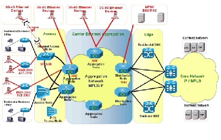
Cisco's Mobile Transport over Pseudowire (MToP) solution builds an MPLS cloud between the distribution nodes (between access and aggregation), and the aggregation nodes on the network edge. The MPLS network is also extended over the point-to-point links from the distribution nodes either via Ethernet, serial, microwave, or a Layer 2 access network. Figure 26-1 provides an example of a Prime Network MToP solution.
The following topics describe the Mobile Transport over Packet (MToP) services and properties you can view in the Vision client. If you cannot perform an operation that is described in these topics, you may not have sufficient permissions; see Permissions for Managing MToP.
- Viewing SAToP Pseudowire Type in Logical Inventory
- Viewing CESoPSN Pseudowire Type in Logical Inventory
- Viewing Virtual Connection Properties
- Viewing IMA Group Properties
- Viewing TDM Properties
- Viewing Channelization Properties
- Viewing MLPPP Properties
- Viewing MLPPP Link Properties
- Viewing MPLS Pseudowire Over GRE Properties
- Network Clock Service Overview
- Viewing CEM and Virtual CEM Properties
- Configuring SONET
- Configuring Clock
- Configuring TDM and Channelization
- Configuring Automatic Protection Switching (APS)
Viewing SAToP Pseudowire Type in Logical Inventory
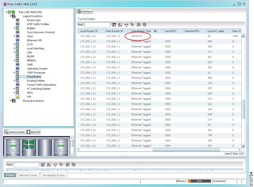
Structure-Agnostic Time Division Multiplexing (TDM) over Packet (SAToP) enables the encapsulation of TDM bit-streams (T1, E1, T3, or E3) as pseudowires over PSNs. As a structure-agnostic protocol, SAToP disregards any structure that might be imposed on the signals and TDM framing is not allowed.
To view the SAToP pseudowire type in logical inventory:
Step 1![]() In the Vision client, right-click the device on which SAToP is configured, then choose Inventory.
In the Vision client, right-click the device on which SAToP is configured, then choose Inventory.
Step 2![]() In the Inventory window, choose Logical Inventory > Pseudowires.
In the Inventory window, choose Logical Inventory > Pseudowires.
Step 3![]() In the Tunnel Edges table, select the required entry and scroll horizontally until you see the Pseudowire Type column. See Figure 26-2.
In the Tunnel Edges table, select the required entry and scroll horizontally until you see the Pseudowire Type column. See Figure 26-2.

Note![]() You can also view this information by right-clicking the entry in the table and choosing Properties.
You can also view this information by right-clicking the entry in the table and choosing Properties.
Figure 26-2 SAToP Pseudowire Type in Logical Inventory
Step 4![]() To view the physical inventory for the port, click the hypertext port link.
To view the physical inventory for the port, click the hypertext port link.
Viewing CESoPSN Pseudowire Type in Logical Inventory
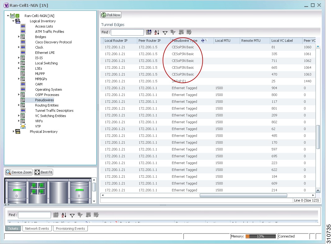
Circuit Emulation Services over PSN (CESoPSN) is a method for encapsulating structured (NxDS0) TDM signals as pseudowires over packet-switching networks, complementary to SAToP. By emulating NxDS0 circuits, CESoPSN:
To view TDM properties for Circuit Emulation (CEM) groups in the Vision client:
Step 1![]() In the Vision client, right-click the device on which CESoPSN is configured, then choose Inventory.
In the Vision client, right-click the device on which CESoPSN is configured, then choose Inventory.
Step 2![]() In the Inventory window, choose Logical Inventory > Pseudowires.
In the Inventory window, choose Logical Inventory > Pseudowires.
Step 3![]() In the Tunnel Edges table, select the required entry and scroll horizontally until you see the Pseudowire Type column. See Figure 26-3.
In the Tunnel Edges table, select the required entry and scroll horizontally until you see the Pseudowire Type column. See Figure 26-3.
Note![]() You can also view this information by right-clicking the entry in the table and choosing Properties.
You can also view this information by right-clicking the entry in the table and choosing Properties.
Figure 26-3 CESoPSN Pseudowire Type in Logical Inventory
Step 4![]() To view the physical inventory for the port, click the hypertext port link.
To view the physical inventory for the port, click the hypertext port link.
Viewing Virtual Connection Properties
The following topics describe how to view properties related to virtual connections:
- Viewing ATM Virtual Connection Cross-Connects
- Viewing ATM VPI and VCI Properties
- Viewing Encapsulation Information
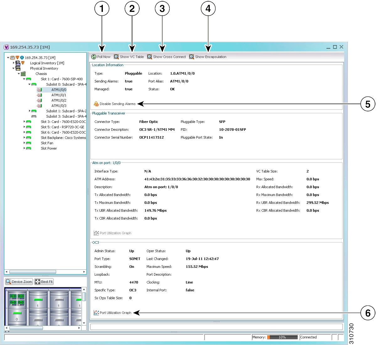
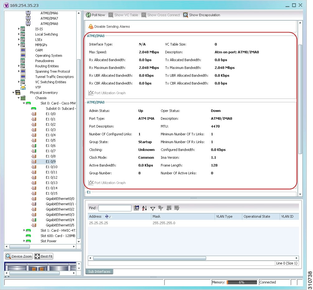
Buttons for viewing these properties are available at the top of the physical inventory window for the selected interface, as shown in Figure 26-4.
Figure 26-4 ATM-Related Properties Available in Physical Inventory
|
|
||
|
|
Displays virtual circuit (VC) information for the selected port.. For more information, see Viewing ATM VPI and VCI Properties. |
|
|
|
Displays cross-connect information for incoming and outgoing ports. For more information, see Viewing ATM Virtual Connection Cross-Connects. |
|
|
|
Displays encapsulation information for incoming and outgoing traffic for the selected item. For more information, see Viewing Encapsulation Information. |
|
|
|
Enables you to manage the alarms on a port. For more information, see Viewing Port Status and Properties and Checking Port Utilization. |
|
|
|
Displays the selected port traffic statistics: Rx/Tx Rate and Rx/Tx Rate History. For more information, see Checking a Port’s Utilization. |
|
|
|
Displays data-link connection identifier (DCLI) information for the selected port. |
Viewing ATM Virtual Connection Cross-Connects
ATM networks are based on virtual connections over a high-bandwidth medium. By using cross-connects to interconnect virtual path or virtual channel links, it is possible to build an end-to-end virtual connection.
An ATM cross-connect can be mapped at either of the following levels:
- Virtual path—Cross-connecting two virtual paths maps one Virtual Path Identifier (VPI) on one port to another VPI on the same port or a different port.
- Virtual channel—Cross-connecting at the virtual channel level maps a Virtual Channel Identifier (VCI) of one virtual channel to another VCI on the same virtual path or a different virtual path.
Cross-connect tables translate the VPI and VCI connection identifiers in incoming ATM cells to the VPI and VCI combinations in outgoing ATM cells. For information about viewing VPI and VCI properties, see Viewing ATM VPI and VCI Properties.
To view ATM virtual connection cross-connects:
Step 1![]() In the Vision client, right-click the required device, then choose Inventory.
In the Vision client, right-click the required device, then choose Inventory.
Step 2![]() Open the VC Cross Connect table in either of the following ways:
Open the VC Cross Connect table in either of the following ways:
- In the Inventory window, choose Logical Inventory > VC Switching Entities > VC Switching Entity. The Cross-Connect Table is displayed in the content pane as shown in Figure 26-5.
- In the Inventory window:
a. Choose Physical Inventory > Chassis > Slot > Subslot > Port.
b. Click the Show Cross Connect button.
The VC Cross Connections window is displayed and contains the same information as the Cross-Connect Table in logical inventory.
Step 3![]() Select an entry and scroll horizontally until you see the required information.
Select an entry and scroll horizontally until you see the required information.
Figure 26-5 ATM Virtual Connection Cross-Connect Properties
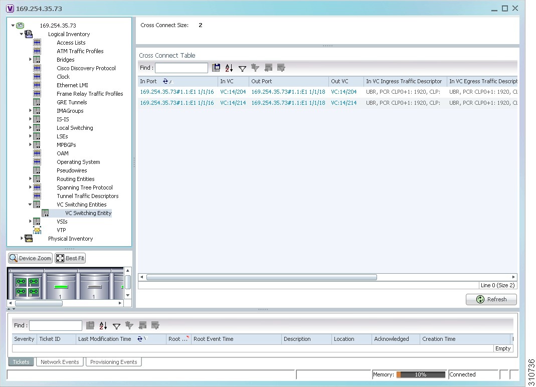
Table 26-1 identifies the properties that are displayed for ATM VC cross-connects.
|
|
|
|---|---|
Incoming virtual connection for the cross-connect. You can view additional details about the virtual connection in the following ways: |
|
Outgoing virtual connection for the cross-connect. You can view additional details about the virtual connection in the following ways: |
|
ATM traffic parameters and service categories for the incoming traffic on the incoming VC cross-connect. For information on VC traffic descriptors, see Table 26-2 . |
|
ATM traffic parameters and service categories for the outgoing traffic on the incoming VC cross-connect. For information on VC traffic descriptors, see Table 26-2 . |
|
ATM traffic parameters and service categories for the outgoing traffic on the outgoing VC cross-connect. For information on VC traffic descriptors, see Table 26-2 . |
|
ATM traffic parameters and service categories for the incoming traffic on the outgoing VC cross-connect. For information on VC traffic descriptors, see Table 26-2 . |
Viewing ATM VPI and VCI Properties
If you know the interface or link configured for virtual connection cross-connects, you can view ATM VPI and VCI properties from the physical inventory window or from the link properties window.
To view ATM VPI and VCI properties, open the VC Table window in either of the following ways:
a.![]() In the map view, double-click the element configured for virtual connection cross-connects.
In the map view, double-click the element configured for virtual connection cross-connects.
b.![]() In the Inventory window, choose Physical Inventory > Chassis > Slot > Subslot > Port.
In the Inventory window, choose Physical Inventory > Chassis > Slot > Subslot > Port.
a.![]() In the map or links view, right-click the required ATM link and choose Properties.
In the map or links view, right-click the required ATM link and choose Properties.
b.![]() In the link properties window, click Calculate VCs.
In the link properties window, click Calculate VCs.
c.![]() After the screen refreshes, click either Show Configured or Show Misconfigured to view the virtual connection cross-connects.
After the screen refreshes, click either Show Configured or Show Misconfigured to view the virtual connection cross-connects.
The VC Table window is displayed, as shown in Figure 26-6.
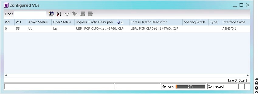
Table 26-3 describes the information displayed in the VC Table window.
|
|
|
|---|---|
Administrative state of the connection: Up, Down, or Unknown. |
|
Traffic parameters and service categories for the incoming traffic. For information on VC traffic descriptors, see Table 26-2 . |
|
Traffic parameters and service categories for the outgoing traffic. For information on VC traffic descriptors, see Table 26-2 . |
|
Viewing Encapsulation Information
To view virtual connection encapsulation information:
Step 1![]() In the Vision client, double-click the element configured for virtual connection encapsulation.
In the Vision client, double-click the element configured for virtual connection encapsulation.
Step 2![]() In the Inventory window, choose Physical Inventory > Chassis > Slot > Subslot > Port.
In the Inventory window, choose Physical Inventory > Chassis > Slot > Subslot > Port.
Step 3![]() Click the Show Encapsulation button.
Click the Show Encapsulation button.
The VC Encapsulation window is displayed as shown in Figure 26-7.
Figure 26-7 VC Encapsulation Properties
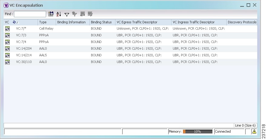
Table 26-4 describes the information displayed in the VC Encapsulation window.
|
|
|
|---|---|
Type of encapsulation, such as Point-to-Point Protocol (PPP) over ATM (PPPoA) or ATM adaption layer Type 5 (AAL5). |
|
Information tied to the virtual connection, such as a username. |
|
Traffic parameters and service categories for the outgoing traffic. For information on VC traffic descriptors, see Table 26-2 . |
|
Traffic parameters and service categories for the incoming traffic. For information on VC traffic descriptors, see Table 26-2 . |
|
Viewing IMA Group Properties
Step 1![]() In the Vision client, double-click the required device.
In the Vision client, double-click the required device.
Step 2![]() In the Inventory window, choose Logical Inventory > IMA Groups > group. IMA group properties and the IMA Members table are displayed in the content pane as shown in Figure 26-8.
In the Inventory window, choose Logical Inventory > IMA Groups > group. IMA group properties and the IMA Members table are displayed in the content pane as shown in Figure 26-8.
Figure 26-8 IMA Group Properties
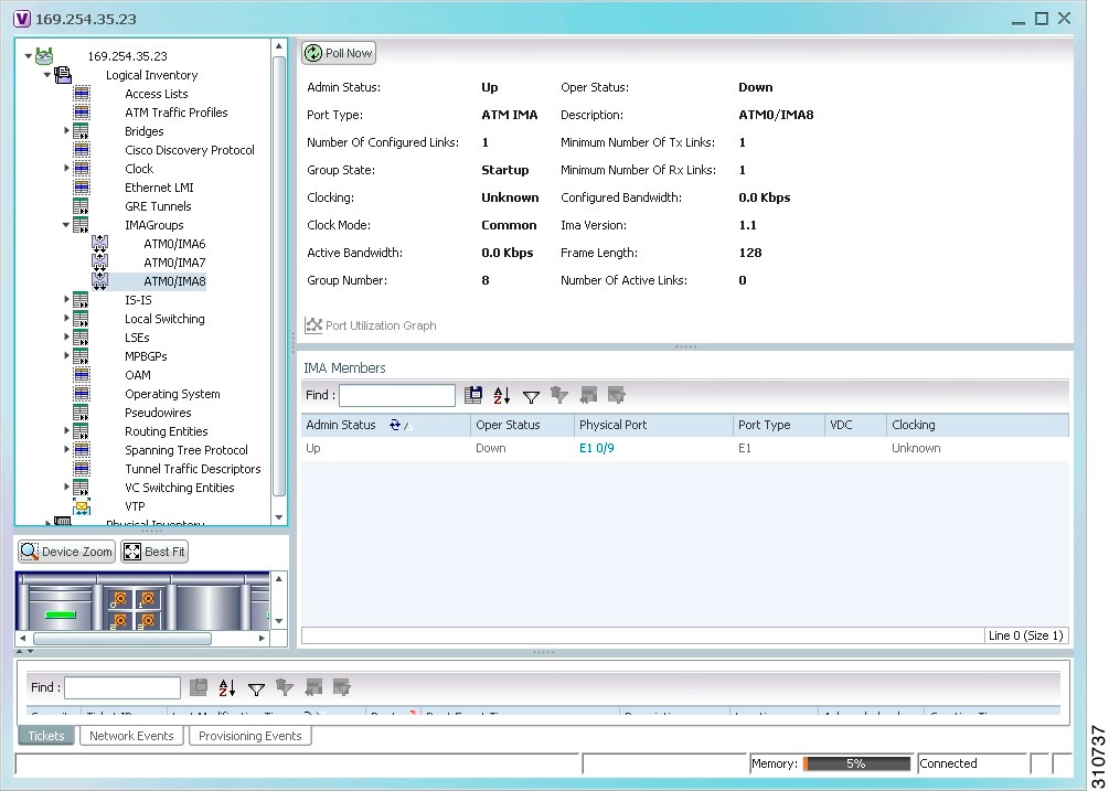
Table 26-5 describes the information displayed for the IMA group.
Table 26-6 describes the information displayed in the IMA Members table.
Step 3![]() In the IMA Members table, click a hyperlinked port entry to view the port properties in physical inventory. See Figure 26-9.
In the IMA Members table, click a hyperlinked port entry to view the port properties in physical inventory. See Figure 26-9.
The information that is displayed for the port in physical inventory depends on the type of connection, such as SONET or ATM.
Figure 26-9 ATM IMA Port in Physical Inventory
Viewing TDM Properties
TDM is a mechanism for combining two or more slower-speed data streams into a single high-speed communication channel. In this model, data from multiple sources is divided into segments that are transmitted in a defined sequence. Each incoming data stream is allocated a timeslot of a fixed length, and the data from each stream is transmitted in turn. For example, data from data stream 1 is transmitted during timeslot 1, data from data stream 2 is transmitted during timeslot 2, and so on. After each incoming stream has transmitted data, the cycle begins again with data stream 1. The transmission order is maintained so that the input streams can be reassembled at the destination.
MToP encapsulates TDM streams for delivery over packet-switching networks (PSNs) using the following methods:
- SAToP—A method for encapsulating TDM bit-streams (T1, E1, T3, or E3) as pseudowires over PSNs.
- CESoPSN—A method for encapsulating structured (NxDS0) TDM signals as pseudowires over PSNs.
For T1 or E1 entries, the TDM properties presented in Table 26-7 are displayed in physical inventory in addition to the existing T1 or E1 properties.
Viewing Channelization Properties
Prime Network supports the channelization of SONET/SDH and T3 5.0. When a line is channelized, it is logically divided into smaller bandwidth channels called paths. These paths (referred to as high order paths or HOPs) can, in turn, contain low order paths, or LOPs. The sum of the bandwidth on all paths cannot exceed the line bandwidth.
For SONET show and configuration commands, see Configuring SONET.
The following topics describe how to view channelization properties for SONET/SDH and T3 5.0:
Viewing SONET/SDH Channelization Properties
SONET and SDH use the same concepts for channelization, but the terminology differs. Table 26-8 describes the equivalent terms for SONET and SDH channelization. The information displayed in the Vision client reflects whether SONET or SDH is configured on the interface.
|
|
|
|
|---|---|---|
To view SONET/SDH channelization properties:
Step 1![]() In the Vision client, right-click the required device, then choose Inventory.
In the Vision client, right-click the required device, then choose Inventory.
Step 2![]() Choose Physical Inventory > Chassis > slot > subslot > SONET/SDH-interface. The properties for SONET/SDH and OC-3 are displayed in the content pane. See Figure 26-10.
Choose Physical Inventory > Chassis > slot > subslot > SONET/SDH-interface. The properties for SONET/SDH and OC-3 are displayed in the content pane. See Figure 26-10.
Figure 26-10 SONET/SDH Interface in Physical Inventory
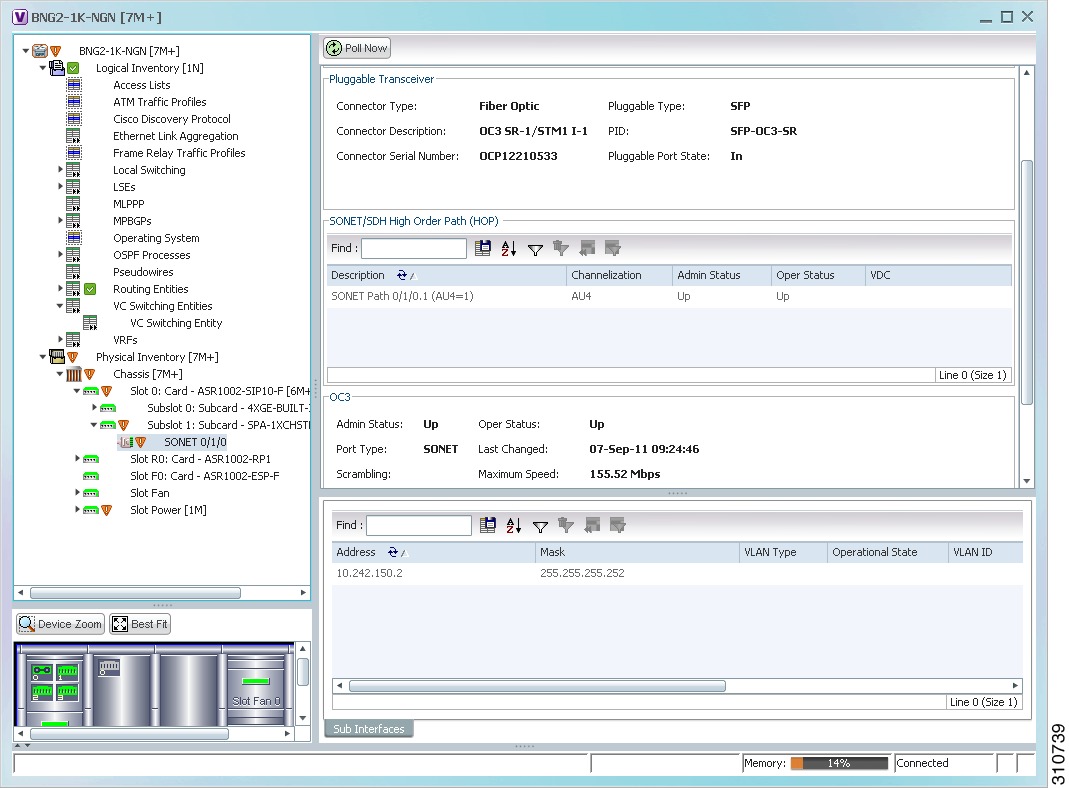
Table 26-9 describes the information that is displayed for SONET/SDH and OC3 in the content pane.
Step 3![]() To view additional information about a channelized path, double-click the required entry in the Description column. The SONET/SDH High Order Path Properties window is displayed as shown in Figure 26-11.
To view additional information about a channelized path, double-click the required entry in the Description column. The SONET/SDH High Order Path Properties window is displayed as shown in Figure 26-11.
Figure 26-11 SONET/SDH High Order Path Properties Window
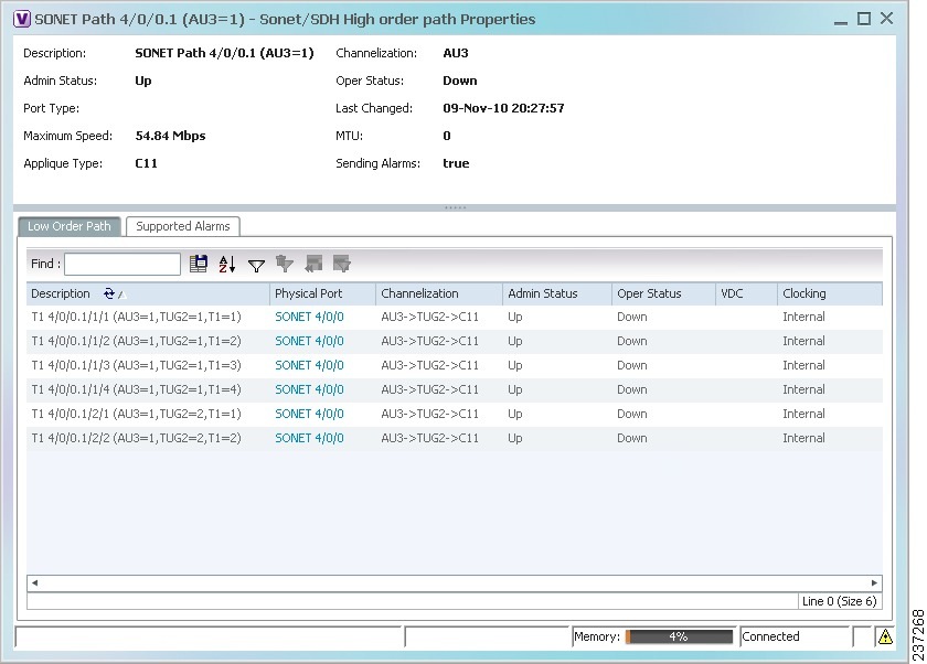
Table 26-10 describes the information displayed in SONET/SDH High Order Path Properties window.
Viewing T3 DS1 and DS3 Channelization Properties
To view T3 DS1 and DS3 channelization properties:
Step 1![]() In the Vision client, right-click the required device, then choose Inventory.
In the Vision client, right-click the required device, then choose Inventory.
Step 2![]() Choose Physical Inventory > Chassis > slot > subslot > T3-interface.
Choose Physical Inventory > Chassis > slot > subslot > T3-interface.
Figure 26-12 shows DS1 channelization properties for T3 in physical inventory.
Figure 26-12 T3 DS1 Channelization Properties in Physical Inventory
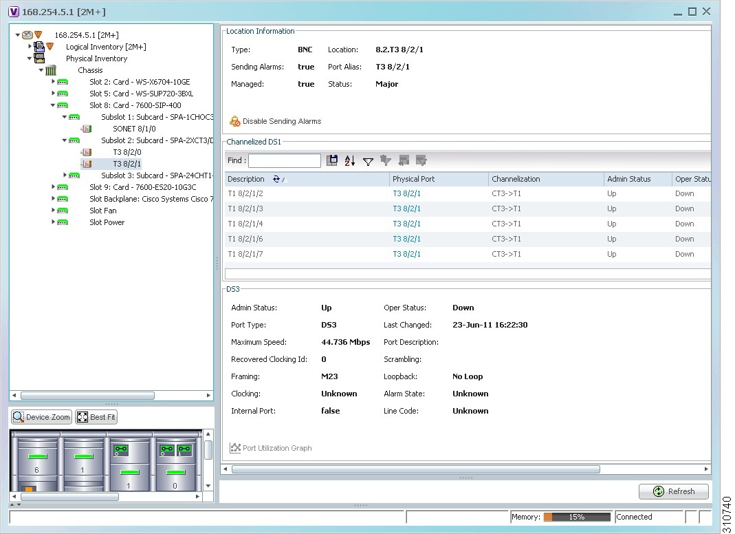
Table 26-11 describes the information that is displayed for Channelized DS1 and DS3 in the content pane.
Step 3![]() To view additional information about a DS1channelized path, double-click the required entry in the Channelized DS1 table. Figure 26-13 shows the information that is displayed in the Channelized DS1 PDH Properties window.
To view additional information about a DS1channelized path, double-click the required entry in the Channelized DS1 table. Figure 26-13 shows the information that is displayed in the Channelized DS1 PDH Properties window.
Figure 26-13 Channelized DS1 PDH Properties Window
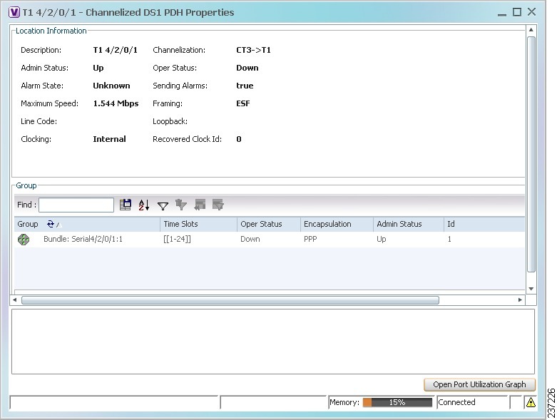
Table 26-12 describes the information that is displayed in the Channelized DS1 PDH Properties window.
Viewing MLPPP Properties
Multilink PPP (MLPPP) is a protocol that connects multiple links between two systems as needed to provide bandwidth when needed. MLPPP packets are fragmented, and the fragments are sent at the same time over multiple point-to-point links to the same remote address. MLPPP provides bandwidth on demand and reduces transmission latency across WAN links.
Step 1![]() In the Vision client, right-click the required device, then choose Inventory.
In the Vision client, right-click the required device, then choose Inventory.
Step 2![]() In the Inventory window, choose Logical Inventory > MLPPP. See Figure 26-14.
In the Inventory window, choose Logical Inventory > MLPPP. See Figure 26-14.
Figure 26-14 MLPPP Properties in Logical Inventory
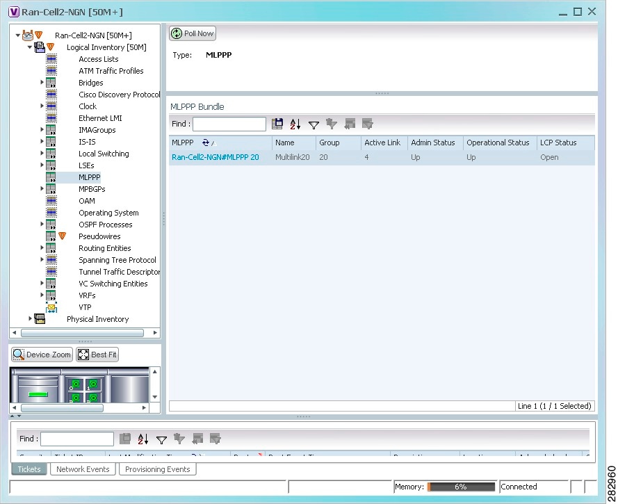
Table 26-13 describes the information that is displayed for MLPPP.
|
|
|
|---|---|
|
|
|
MLPPP bundle name, hyperlinked to the MLPPP Properties window. |
|
Link Control Protocol (LCP) status of the MLPPP bundle: Closed, Open, Started, or Unknown. |
|
Step 3![]() To view properties for individual MLPPP bundles, double-click the hyperlinked entry in the MLPPP Bundle table.
To view properties for individual MLPPP bundles, double-click the hyperlinked entry in the MLPPP Bundle table.
Table 26-14 describes the information that is displayed in the MLPPP Properties window.
Step 4![]() To view the interface properties in physical inventory, double-click the required entry in the ID column.
To view the interface properties in physical inventory, double-click the required entry in the ID column.
Viewing MLPPP Link Properties
An MLPPP link is a link that connects two MLPPP devices.
To view MLPPP link properties:
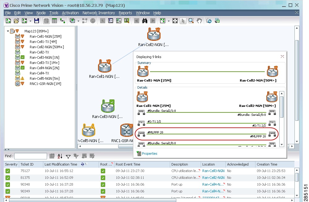
Step 1![]() In the Vision client map view, select a link connected to two MLPPP devices and open the link quick view window as shown in Figure 26-15.
In the Vision client map view, select a link connected to two MLPPP devices and open the link quick view window as shown in Figure 26-15.
Figure 26-15 MLPPP Link in Link Quick View
Step 2![]() In the link quick view window, click Properties.
In the link quick view window, click Properties.
Step 3![]() In the link properties window, select the MLPPP link. The link properties are displayed as shown in Figure 26-16.
In the link properties window, select the MLPPP link. The link properties are displayed as shown in Figure 26-16.
Figure 26-16 MLPPP Link Properties
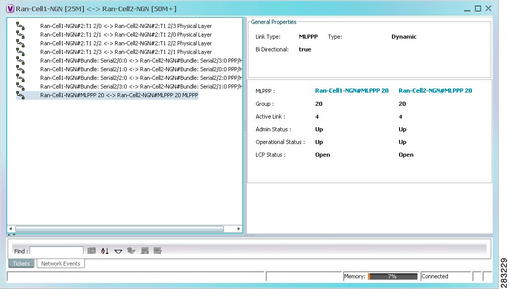
Table 26-15 describes the information that is displayed for the MLPPP link.
Viewing MPLS Pseudowire Over GRE Properties
Generic routing encapsulation (GRE) is a tunneling protocol, originated by Cisco Systems and standardized in RFC 2784. GRE encapsulates a variety of network layer packets inside IP tunneling packets, creating a virtual point-to-point link to devices at remote points over an IP network. GRE encapsulates the entire original packet with a standard IP header and GRE header before the IPsec process. GRE can carry multicast and broadcast traffic, making it possible to configure a routing protocol for virtual GRE tunnels.
In RAN backhaul networks, GRE is used to transport cell site traffic across IP networks (nonMPLS). In addition, GRE tunnels can be used to transport TDM traffic (TDMoMPLSoGRE) as part of the connectivity in the following sample scenarios:
- Among cell site-facing Cisco 7600 routers and base station controller (BSC) site-facing Cisco 7600 routers.
- Between a Cisco Mobile Wireless Router (MWR) device and a BSC site-facing Cisco 7600 router.
Using GRE tunnels to transport Any Traffic over MPLS (AToM) enables mobile service providers to deploy AToM pseudowires in a network where MPLS availability is discontinuous; for example, in networks where the pseudowire endpoints are located in MPLS edge routers with a plain IP core network, or where two separate MPLS networks are connected by a transit network with plain IP forwarding.
To view the properties for MPLS pseudowire over GRE:
Step 1![]() In the Vision client, right-click the required device, then choose Inventory.
In the Vision client, right-click the required device, then choose Inventory.
Step 2![]() In the Inventory window, choose Logical Inventory > Pseudowires. The Tunnel Edges table is displayed in the content pane as shown in Figure 26-17.
In the Inventory window, choose Logical Inventory > Pseudowires. The Tunnel Edges table is displayed in the content pane as shown in Figure 26-17.
Step 3![]() Select the required entry and scroll horizontally until you see the required information.
Select the required entry and scroll horizontally until you see the required information.
Figure 26-17 MPLS Pseudowire Tunnels over GRE Properties
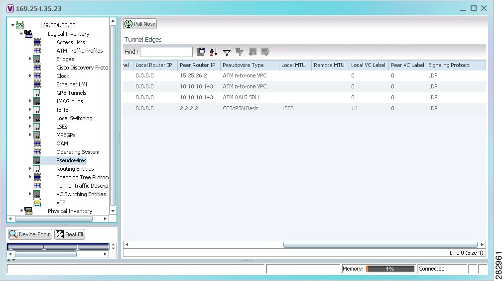
Table 26-16 describes the information included in the Tunnel Edges table specifically for MPLS pseudowire tunnels over GRE.
|
|
|
|---|---|
Path to be used for MPLS pseudowire traffic. Click the hyperlinked entry to view the tunnel details in logical inventory. |
Step 4![]() To view GRE Tunnel properties, choose Logical Inventory > GRE Tunnels.
To view GRE Tunnel properties, choose Logical Inventory > GRE Tunnels.
Figure 26-18 shows the Tunnel Edges table that is displayed for GRE tunnels.
Figure 26-18 GRE Tunnel Properties in Logical Inventory
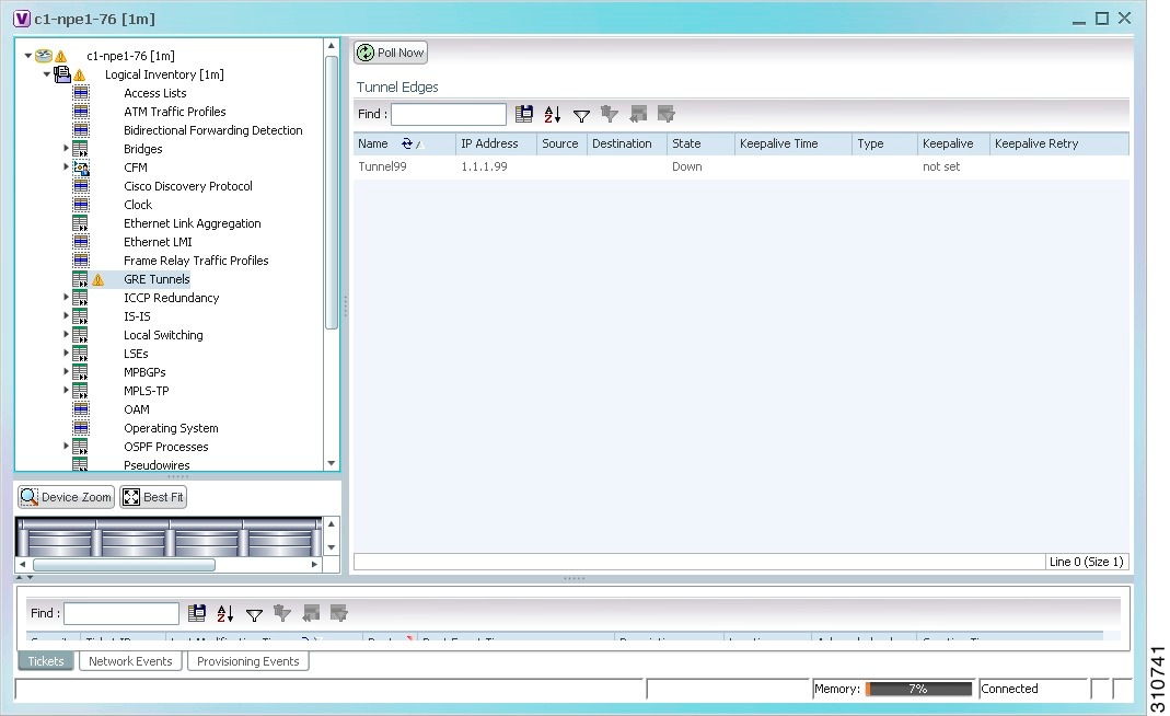
Table 26-17 describes the information that is displayed for GRE tunnels in logical inventory.
Network Clock Service Overview
Network clock service refers to the means by which a clock signal is generated or derived and distributed through a network and its individual nodes for the purpose of ensuring synchronized network operation. Network clocking is particularly important for mobile service providers to ensure proper transport of cellular traffic from cell sites to Base Station Control (BSC) sites.
Note![]() In Prime Network, clock service refers to network clock service.
In Prime Network, clock service refers to network clock service.
The following topics describe how to use the Vision client to monitor clock service:
- Monitoring Clock Service
- Monitoring PTP Service
- Viewing Pseudowire Clock Recovery Properties
- Viewing SyncE Properties
- Applying a Network Clock Service Overlay
- Viewing CEM and Virtual CEM Properties
Monitoring Clock Service
Step 1![]() In the Vision client, right-click the required device, then choose Inventory.
In the Vision client, right-click the required device, then choose Inventory.
Step 2![]() In the Inventory window, choose Logical Inventory > Clock. Clock service information is displayed in the content pane as shown in Figure 26-19.
In the Inventory window, choose Logical Inventory > Clock. Clock service information is displayed in the content pane as shown in Figure 26-19.
Figure 26-19 Clock Service Properties
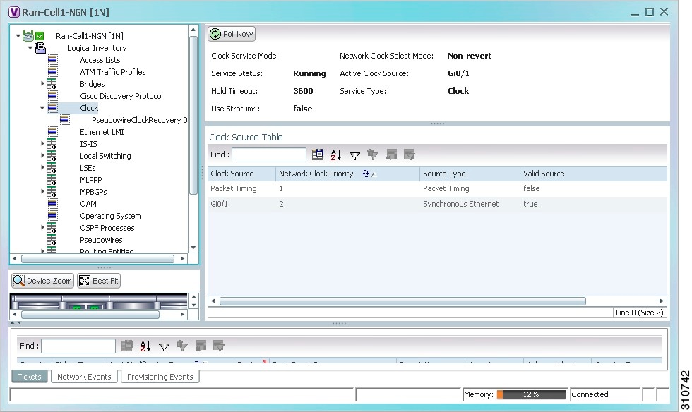
Table 26-18 describes the information displayed for clocking service.
Monitoring PTP Service
In networks that employ TDM, periodic synchronization of device clocks is required to ensure that the receiving device knows which channel is which for accurate reassembly of the data stream. The Precision Time Protocol (PTP) standard:
- Specifies a clock synchronization protocol that enables this synchronization.
- Applies to distributed systems that consist of one or more nodes communicating over a network.
Defined by IEEE 1588-2008, PTP Version 2 (PTPv2) allows device synchronization at the nanosecond level.
PTP uses the concept of master and slave devices to achieve precise clock synchronization. Using PTP, the master device periodically starts a message exchange with the slave devices. After noting the times at which the messages are sent and received, each slave device calculates the difference between its system time and the system time of the master device. The slave device then adjusts its clock so that it is synchronized with the master device. When the master device initiates the next message exchange, the slave device again calculates the difference and adjusts its clock. This repetitive synchronization ensures that device clocks are coordinated and that data stream reassembly is accurate. For configuring PTP, see Configuring SONET.
Step 1![]() In the Vision client, right-click the required device, then choose Inventory.
In the Vision client, right-click the required device, then choose Inventory.
Step 2![]() In the Inventory window, choose Logical Inventory > Clock > PTP Service. The PTP service properties are displayed in the content pane as shown in Figure 26-20.
In the Inventory window, choose Logical Inventory > Clock > PTP Service. The PTP service properties are displayed in the content pane as shown in Figure 26-20.
Figure 26-20 PTP Service Properties
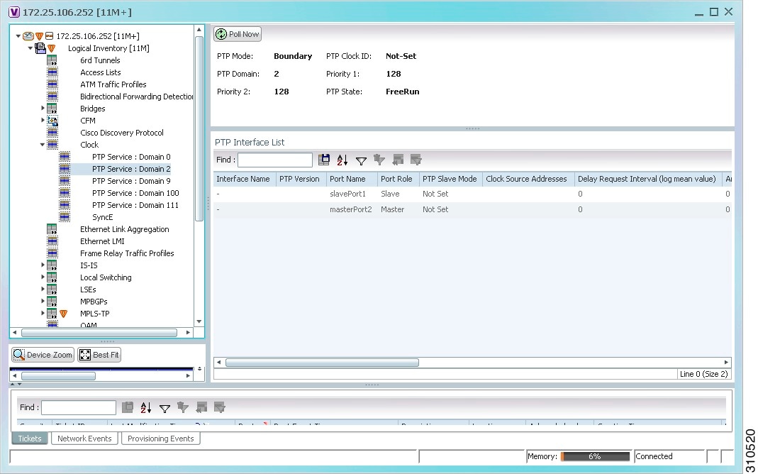
Table 26-19 describes the properties that are displayed for PTP service.
|
|
|
|---|---|
Number of the domain used for PTP traffic. A single network can contain multiple separate domains. |
|
First value checked for clock selection. The clock with the lowest priority takes precedence. |
|
If two or more clocks have the same value in the Priority 1 field, the value in this field is used for clock selection. |
|
Clock state according to the PTP engine:
PTP clock status syslog support—As part of the syslog support, Prime Network started supporting PTP clock status syslog besides the PTP inventory information. While receiving the syslog, Prime Network queries the device, and receives the PTP state information and updates in the respective PTP service. The service alarm supported for the PTP status information is PTP port clock state change alarm. Theses service alarms and the syslogs are correlated under the PTP service as clock service. For more information on PTP clock status update service alarm, refer Cisco Prime Network Supported Service Alarms. |
|
|
|
|
Version of PTP used. The default value is 2, indicating PTPv2. |
|
For an interface defined as a slave device, the mode used for PTP clocking: |
|
When the interface is in PTP master mode, the interval specified to member devices for delay request messages. The intervals use base 2 values, as follows:
|
|
Interval value for PTP announcement packets:
|
|
Number of PTP announcement intervals before the session times out. Values are 2-10. |
|
Interval for sending PTP synchronization messages:
|
|
Maximum clock offset value, in nanoseconds, before PTP attempts to resynchronize. |
|
Physical interface identifier, hyperlinked to the routing information for the interface. |
|
For an interface defined as a master device, the mode used for PTP clocking:
|
|
IP addresses of the clock destinations. This field contains IP addresses only when Master mode is enabled. |
|
Viewing Pseudowire Clock Recovery Properties
To view pseudowire clock recovery properties:
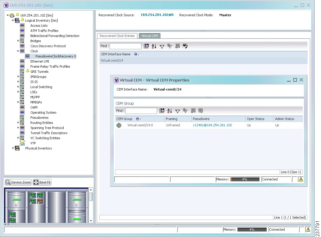
Step 1![]() Choose Logical Inventory > Clock > Pseudowire Clock Recovery. The Vision client displays the Virtual CEM information by default. See Figure 26-21.
Choose Logical Inventory > Clock > Pseudowire Clock Recovery. The Vision client displays the Virtual CEM information by default. See Figure 26-21.
Figure 26-21 Pseudowire Clock Recovery - Virtual CEM Tab
Step 2![]() To view more information about a virtual CEM, right-click the virtual CEM, then choose Properties. The Virtual CEM Properties window is displayed.
To view more information about a virtual CEM, right-click the virtual CEM, then choose Properties. The Virtual CEM Properties window is displayed.
The information that is displayed in the Virtual CEM Properties window depends on whether or not the virtual CEM belongs to a group:
- If a CEM group is not configured on the virtual CEM, the Virtual CEM Properties window contains only the CEM interface name.
- If a CEM group is configured on the virtual CEM, the Virtual CEM Properties window contains the information described in Table 26-20 .
|
|
|
|---|---|
|
|
|
Name of the pseudowire configured on the CEM interface, hyperlinked to the pseudowire properties in logical inventory. |
|
Step 3![]() To view additional CEM group properties, double-click the required CEM group.
To view additional CEM group properties, double-click the required CEM group.
Table 26-21 describes the information displayed in the CEM Group Properties window.
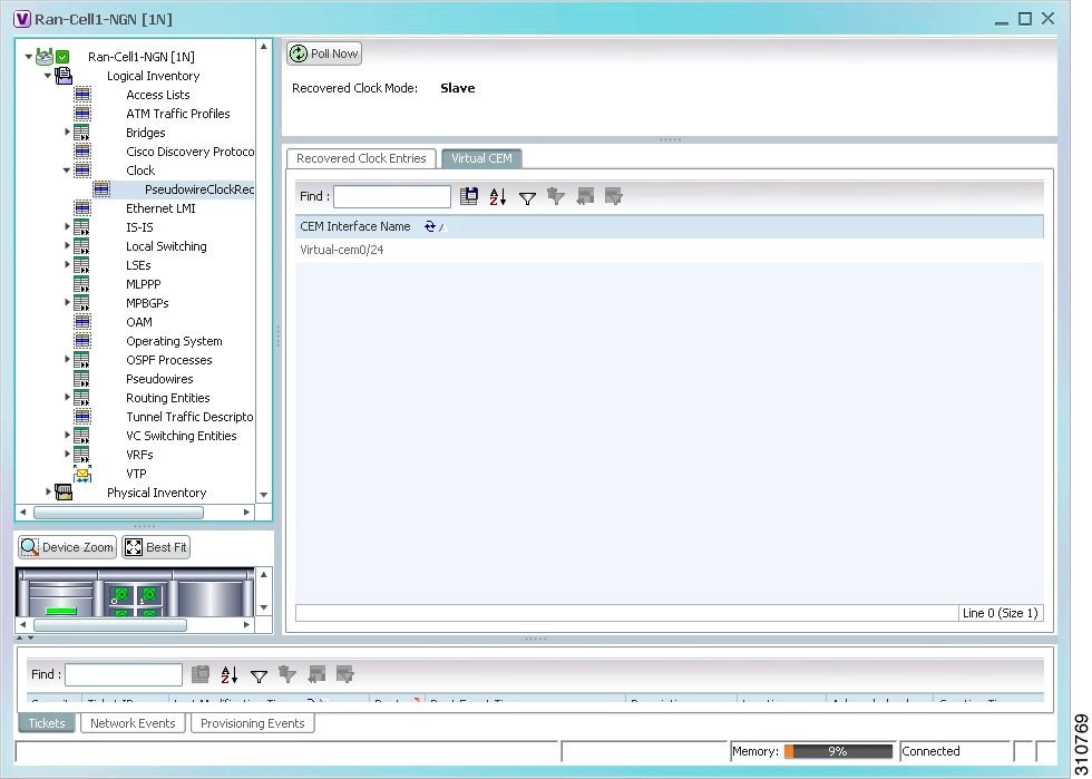
Step 4![]() To view recovered clock entries, click the Recovered Clock Entries tab. See Figure 26-22.
To view recovered clock entries, click the Recovered Clock Entries tab. See Figure 26-22.
If no recovered clock entries exist, this tab is not displayed.
Figure 26-22 Pseudowire Clock Recovery - Recovered Clock Entries Tab
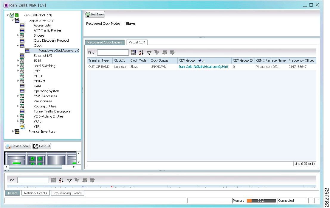
Table 26-22 describes the information displayed for pseudowire clock recovery.
Viewing SyncE Properties
With Ethernet equipment gradually replacing SONET and SDH equipment in service-provider networks, frequency synchronization is required to provide high-quality clock synchronization over Ethernet ports. Synchronous Ethernet (SyncE), a recently adopted standard, provides the required synchronization at the physical level.
In SyncE, Ethernet links are synchronized by timing their bit clocks from high-quality, stratum-1-traceable clock signals in the same manner as SONET/SDH. Operations messages maintain SyncE links, and ensure a node always derives timing from the most reliable source.
For configuring SyncE, see Configuring Clock. To view SyncE properties, choose Logical Inventory > Clock > SyncE. (See Figure 26-23.)
Figure 26-23 SyncE Properties in Logical Inventory
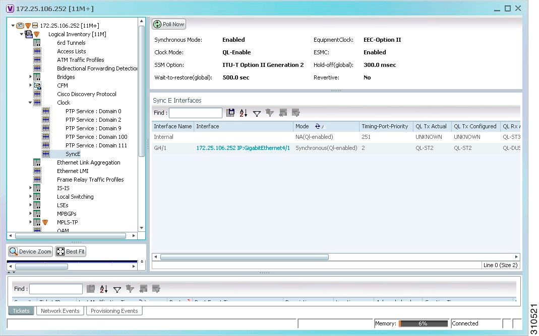
Table 26-23 describes the information that is displayed for SyncE.
|
|
|
|---|---|
Status of the automatic synchronization selection process: Enabled or Disable. |
|
Ethernet Equipment Clock (EEC) options: EEC-Option I or EEC-Option II. |
|
Whether the clock is enabled or disabled for the Quality Level (QL) function: QL-Enabled or QL-Disabled. |
|
Ethernet Synchronization Message Channel (ESMC) status: Enabled or Disabled. |
|
Length of time (in milliseconds) to wait before issuing a protection response to a failure event. |
|
Length of time (in seconds) to wait after a failure is fixed before the span returns to its original state. |
|
Whether the network clock is to use revertive mode: Yes or No. |
|
|
|
|
Name of the Gigabit or 10 Gigabit interface associated with SyncE. If SyncE is not associated with a Gigabit or 10 Gigabit interface, this field contains Internal. |
|
Hyperlinked entry to the interface routing information in the Routing Entity Controller window. For more information, see Viewing Routing Entities. |
|
Whether the interface is enabled or disabled for the QL function: QL-Enabled or QL-Disabled. |
|
Value used for selecting a SyncE interface for clocking if more than one interface is configured. Values are from 1 to 250, with 1 being the highest priority. |
|
Actual type of outgoing quality level information, depending on the globally configured SSM option:
|
|
Configured type of outgoing quality level information, depending on the globally configured SSM option. See QL Tx Actual for the available values. |
|
Actual type of incoming quality level information, depending on the globally configured SSM option. See QL Tx Actual for the available values. |
|
Configured type of incoming quality level information, depending on the globally configured SSM option. See QL Tx Actual for the available values. |
|
Length of time (in milliseconds) to wait after a clock source goes down before removing the source. |
|
Length of time (in seconds) to wait after a failure is fixed before the interface returns to its original state. |
|
Whether ESMC is enabled for outgoing QL information on the interface: Enabled, Disabled, or NA (Not Available). |
|
Whether ESMC is enabled for incoming QL information on the interface: Enabled, Disabled, or NA (Not Available). |
|
Whether SSM is enabled for outgoing QL information on the interface: Enabled, Disabled, or NA (Not Available). |
|
Whether SSM is enabled for incoming QL information on the interface: Enabled, Disabled, or NA (Not Available). |
|
Applying a Network Clock Service Overlay
A service overlay allows you to isolate the parts of a network that are being used by a particular service. This information can then be used for troubleshooting. For example, the overlay can highlight configuration or design problems when bottlenecks occur and all the site interlinks use the same link.
To apply a network clock overlay:
Step 1![]() In the Vision client, display the network map on which you want to apply an overlay.
In the Vision client, display the network map on which you want to apply an overlay.
Step 2![]() From the main toolbar, click Choose Overlay Type and choose Network Clock.
From the main toolbar, click Choose Overlay Type and choose Network Clock.
The Select Network Clock Service Overlay dialog box is displayed.
Step 3![]() Do one of the following:
Do one of the following:
The search condition is “contains.” Search strings are case-insensitive. For example, if you choose the Name category and enter “net,” the Vision client displays VPNs “net” and “NET” in the names whether net appears at the beginning, middle, or at the end of the name: for example, Ethernet.
Step 4![]() Select the network clock service overlay that you want to apply to the map.
Select the network clock service overlay that you want to apply to the map.
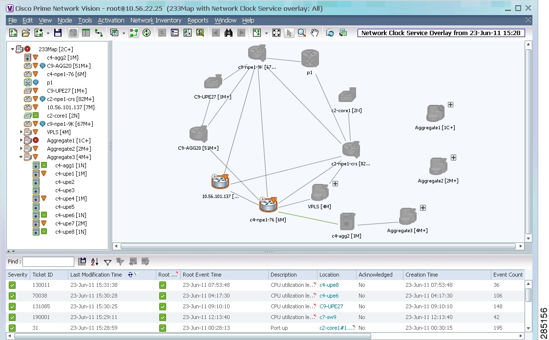
The elements and links used by the selected network clock are highlighted in the map, and the overlay name is displayed in the title of the window. (See Figure 26-24.)
Figure 26-24 Network Clock Service Overlay Example
In addition, the elements configured for clocking service display a clock service icon as in the following example:

Note![]() An overlay is a snapshot taken at a specific point in time and does not reflect changes that occur in the service. As a result, the information in an overlay can become stale. To update the overlay, click Refresh Overlay in the main toolbar.
An overlay is a snapshot taken at a specific point in time and does not reflect changes that occur in the service. As a result, the information in an overlay can become stale. To update the overlay, click Refresh Overlay in the main toolbar.
Viewing CEM and Virtual CEM Properties
The following topics describe how to view CEM and virtual CEM properties and interfaces:
Viewing CEM Interfaces
Step 1![]() In the Vision client, double-click the required device.
In the Vision client, double-click the required device.
Step 2![]() In the Inventory window, choose Physical Inventory > Chassis > slot > subslot > interface. The CEM interface name is displayed in the content pane as shown in Figure 26-25.
In the Inventory window, choose Physical Inventory > Chassis > slot > subslot > interface. The CEM interface name is displayed in the content pane as shown in Figure 26-25.
Viewing Virtual CEMs
To view virtual CEMs, choose Logical Inventory > Clock > Pseudowire Clock Recovery.
The virtual CEM interfaces are listed in the Virtual CEM tab.
Viewing CEM Groups
CEM groups can be configured on physical or virtual CEM interfaces. The underlying interface determines where you view CEM group properties in the Vision client:
Viewing CEM Groups on Physical Interfaces
When you configure a CEM group on a physical interface, the CEM group properties are displayed in physical inventory for that interface.
To view CEM groups configured on physical interfaces:
Step 1![]() In the Vision client, double-click the required device.
In the Vision client, double-click the required device.
Step 2![]() In the Inventory window, choose Physical Inventory > Chassis > slot > subslot > interface.
In the Inventory window, choose Physical Inventory > Chassis > slot > subslot > interface.
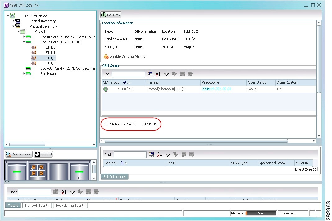
The CEM group information is displayed in the content pane with other interface properties (Figure 26-26).
Figure 26-26 CEM Group Information
See Table 26-20 for a description of the properties displayed for CEM groups in the content pane.
Step 3![]() To view additional information, double-click the required group.
To view additional information, double-click the required group.
The CEM Group Properties window is displayed as shown in Figure 26-27.
Figure 26-27 CEM Group Properties Window
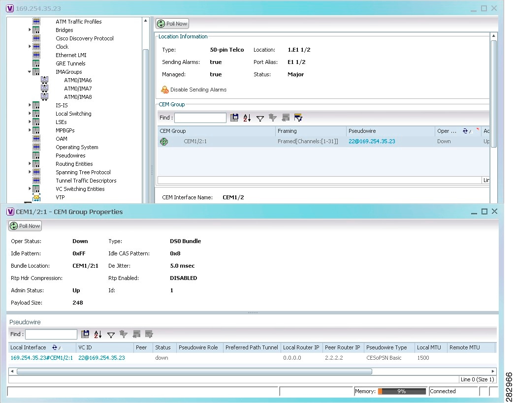
See Table 17-29for the properties displayed in the Pseudowire table in the CEM Group Properties window.
Viewing CEM Groups on Virtual CEM Interfaces
When you configure a CEM group on a virtual CEM, the CEM group information is displayed below the virtual CEM in logical inventory.
To view CEM groups on virtual CEM interfaces:
Step 1![]() In the Vision client, right-click the required device, then choose Inventory.
In the Vision client, right-click the required device, then choose Inventory.
Step 2![]() In the Inventory window, choose Logical Inventory > Clock > Pseudowire Clock Recovery.
In the Inventory window, choose Logical Inventory > Clock > Pseudowire Clock Recovery.
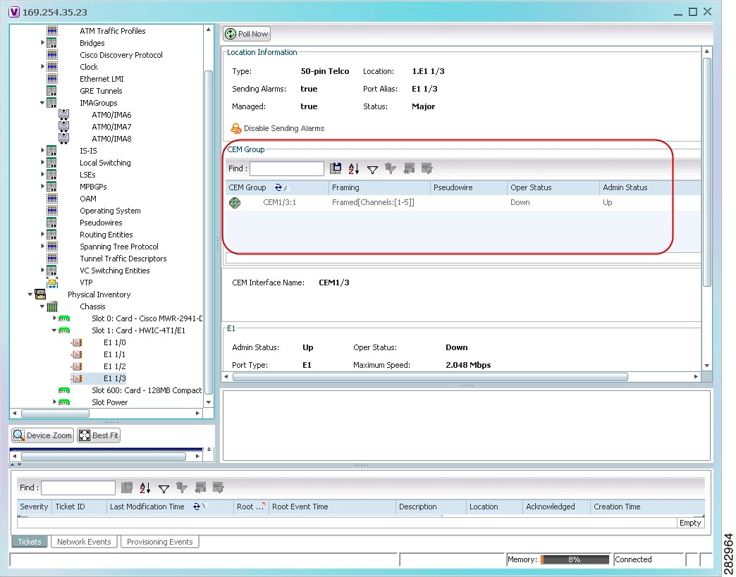
Step 3![]() In the Virtual CEM tab, right-click the CEM interface name and choose Properties. The CEM group properties are displayed in a separate window (Figure 26-28). If a pseudowire is configured on the CEM group for out-of-band clocking, the pseudowire VCID is also shown.
In the Virtual CEM tab, right-click the CEM interface name and choose Properties. The CEM group properties are displayed in a separate window (Figure 26-28). If a pseudowire is configured on the CEM group for out-of-band clocking, the pseudowire VCID is also shown.
Figure 26-28 CEM Group Properties
Step 4![]() To view additional CEM group properties, double-click the required CEM group.
To view additional CEM group properties, double-click the required CEM group.
Table 26-21 describes the information displayed in the CEM Group Properties window.
Configuring SONET
The table below lists the SONET commands can be launched from the inventory by right-clicking a SONET port and selecting Commands > SONET. Your permissions determine whether you can run these commands (see Permissions for Vision Client NE-Related Operations). To find out if a device supports these commands, see the Cisco Prime Network 5.0 Supported Cisco VNEs.
Configuring Clock
With Ethernet equipment gradually replacing SONET and SDH equipment in service-provider networks, frequency synchronization is required to provide high-quality clock synchronization over Ethernet ports. SyncE and PTP are two widely used clock synchronization protocol used in ethernet based networks.
Clocking configuration commands allows you to configure SyncE and PTP clock configuration on Cisco router. SyncE and PTP clocking configuration is predominantly used in RAN Backhaul (or MToP) network where TDM traffic carried from cell site router to central office via packet switched network.
These commands can be launched from the logical inventory by right-clicking on Clock node. Your permissions determine whether you can run these commands (see Permissions for Vision Client NE-Related Operations). To find out if a device supports these commands, see the Cisco Prime Network 5.0 Supported Cisco VNEs.
Configuring TDM and Channelization
The table below lists the supported TDM and channelization commands and how to launch them. Your permissions determine whether you can run these commands (see Permissions for Vision Client NE-Related Operations). To find out if a device supports these commands, see the Cisco Prime Network 5.0 Supported Cisco VNEs.
Configuring Automatic Protection Switching (APS)
APS refers to the mechanism of using a protect interface in the SONET network as the backup for working interface. When the working interface fails, the protect interface quickly assumes its traffic load. The working interfaces and their protect interfaces make up an APS group. SONET APS offers recovery from fiber (external) or equipment (interface and internal) failures at the SONET line layer.
The table below lists the supported APS commands. Your permissions determine whether you can run these commands (see Permissions for Vision Client NE-Related Operations). To find out if a device supports these commands, see the Cisco Prime Network 5.0 Supported Cisco VNEs.
 Feedback