-
null
- Creating Maps
- Access Point Placement
- Creating a Network Design
- Using Chokepoints to Enhance Tag Location Reporting
- Monitoring Maps
- Importing or Exporting WLSE Map Data
- Creating and Applying Calibration Models
- Analyzing Element Location Accuracy Using Testpoints
Adding and Using Maps
This chapter describes how to add maps to the Cisco WCS database and use them to monitor your wireless LAN. It contains these sections:
•![]() Using Chokepoints to Enhance Tag Location Reporting
Using Chokepoints to Enhance Tag Location Reporting
•![]() Importing or Exporting WLSE Map Data
Importing or Exporting WLSE Map Data
•![]() Creating and Applying Calibration Models
Creating and Applying Calibration Models
•![]() Analyzing Element Location Accuracy Using Testpoints
Analyzing Element Location Accuracy Using Testpoints
Creating Maps
With the Cisco WCS database, you can add maps and view your managed system on realistic campus, building, and floor map maps. Follow the instructions in the sections below to add a campus, buildings, outdoor areas, floor plans, and access points to maps in the Cisco WCS database:
Adding a Campus
Follow these steps to add a single campus map to the Cisco WCS database.
Step 1 ![]() Save the map in .PNG, .JPG, .JPEG, or .GIF format.
Save the map in .PNG, .JPG, .JPEG, or .GIF format.

Note ![]() The map can be any size because WCS automatically resizes the map to fit its working areas.
The map can be any size because WCS automatically resizes the map to fit its working areas.
Step 2 ![]() Browse to and import the map from anywhere in your file system.
Browse to and import the map from anywhere in your file system.
Step 3 ![]() Click Monitor > Maps to display the Maps page.
Click Monitor > Maps to display the Maps page.
Step 4 ![]() From the Select a command drop-down menu, choose New Campus and click GO.
From the Select a command drop-down menu, choose New Campus and click GO.
Step 5 ![]() On the Maps > New Campus page, enter the campus name and campus contact name.
On the Maps > New Campus page, enter the campus name and campus contact name.
Step 6 ![]() Browse to and choose the image filename or CAD file containing the map of the campus and click Open.
Browse to and choose the image filename or CAD file containing the map of the campus and click Open.
Step 7 ![]() Check the Maintain Aspect Ratio check box to prevent length and width distortion when WCS resizes the map.
Check the Maintain Aspect Ratio check box to prevent length and width distortion when WCS resizes the map.
Step 8 ![]() Enter the horizontal and vertical span of the map in feet.
Enter the horizontal and vertical span of the map in feet.
Note ![]() The horizontal and vertical span should be larger than any building or floor plan to be added to the campus.
The horizontal and vertical span should be larger than any building or floor plan to be added to the campus.
Step 9 ![]() Click OK to add this campus map to the Cisco WCS database. WCS displays the Maps page, which lists maps in the database, map types, and campus status.
Click OK to add this campus map to the Cisco WCS database. WCS displays the Maps page, which lists maps in the database, map types, and campus status.
Adding Buildings
You can add buildings to the Cisco WCS database regardless of whether you have added campus maps to the database. This section explains how to add a building to a campus map or a standalone building to the Cisco WCS database.
Adding a Building to a Campus Map
Follow these steps to add a building to a campus map in the Cisco WCS database.
Step 1 ![]() Click Monitor > Maps to display the Maps page.
Click Monitor > Maps to display the Maps page.
Step 2 ![]() Click the desired campus. WCS displays the Maps > Campus Name page.
Click the desired campus. WCS displays the Maps > Campus Name page.
Step 3 ![]() From the Select a command drop-down menu, choose New Building and click GO.
From the Select a command drop-down menu, choose New Building and click GO.
Step 4 ![]() On the Campus Name > New Building page, follow these steps to create a virtual building in which to organize related floor plan maps:
On the Campus Name > New Building page, follow these steps to create a virtual building in which to organize related floor plan maps:
a. ![]() Enter the building name.
Enter the building name.
b. ![]() Enter the building contact name.
Enter the building contact name.
c. ![]() Enter the number of floors and basements.
Enter the number of floors and basements.
d. ![]() Enter an approximate building horizontal span and vertical span (width and depth on the map) in feet.
Enter an approximate building horizontal span and vertical span (width and depth on the map) in feet.

Tip ![]() The horizontal and vertical span should be larger than or the same size as any floors that you might add later.You can also use Ctrl-click to resize the bounding area in the upper left corner of the campus map. As you change the size of the bounding area, the Horizontal Span and Vertical Span parameters of the building change to match your actions.
The horizontal and vertical span should be larger than or the same size as any floors that you might add later.You can also use Ctrl-click to resize the bounding area in the upper left corner of the campus map. As you change the size of the bounding area, the Horizontal Span and Vertical Span parameters of the building change to match your actions.
e. ![]() Click Place to put the building on the campus map. WCS creates a building rectangle scaled to the size of the campus map.
Click Place to put the building on the campus map. WCS creates a building rectangle scaled to the size of the campus map.
f. ![]() Click on the building rectangle and drag it to the desired position on the campus map.
Click on the building rectangle and drag it to the desired position on the campus map.
Note ![]() After adding a new building, you can move it from one campus to another without having to recreate it.
After adding a new building, you can move it from one campus to another without having to recreate it.
g. ![]() Click Save to save this building and its campus location to the database. WCS saves the building name in the building rectangle on the campus map.
Click Save to save this building and its campus location to the database. WCS saves the building name in the building rectangle on the campus map.
Note ![]() A hyperlink associated with the building takes you to the corresponding Map page.
A hyperlink associated with the building takes you to the corresponding Map page.
Adding a Standalone Building
Follow these steps to add a standalone building to the Cisco WCS database.
Step 1 ![]() Click Monitor > Maps to display the Maps page.
Click Monitor > Maps to display the Maps page.
Step 2 ![]() From the Select a command drop-down menu, choose New Building and click GO.
From the Select a command drop-down menu, choose New Building and click GO.
Step 3 ![]() On the Maps > New Building page, follow these steps to create a virtual building in which to organize related floor plan maps:
On the Maps > New Building page, follow these steps to create a virtual building in which to organize related floor plan maps:
a. ![]() Enter the building name.
Enter the building name.
b. ![]() Enter the building contact name.
Enter the building contact name.
Note ![]() After adding a new building, you can move it from one campus to another without having to recreate it.
After adding a new building, you can move it from one campus to another without having to recreate it.
c. ![]() Enter the number of floors and basements.
Enter the number of floors and basements.
d. ![]() Enter an approximate building horizontal span and vertical span (width and depth on the map) in feet.
Enter an approximate building horizontal span and vertical span (width and depth on the map) in feet.
Note ![]() The horizontal and vertical span should be larger than or the same size as any floors that you might add later.
The horizontal and vertical span should be larger than or the same size as any floors that you might add later.
e. ![]() Click OK to save this building to the database.
Click OK to save this building to the database.
Adding Outdoor Areas
Follow these steps to add an outdoor area to a campus map.
Note ![]() You can add outdoor areas to a campus map in the Cisco WCS database regardless of whether you have added outdoor area maps to the database.
You can add outdoor areas to a campus map in the Cisco WCS database regardless of whether you have added outdoor area maps to the database.
Step 1 ![]() If you want to add a map of the outdoor area to the database, save the map in .PNG, .JPG, .JPEG, or .GIF format. Then browse to and import the map from anywhere in your file system.
If you want to add a map of the outdoor area to the database, save the map in .PNG, .JPG, .JPEG, or .GIF format. Then browse to and import the map from anywhere in your file system.
Note ![]() You do not need a map to add an outdoor area. You can simply define the dimensions of the area to add it to the database. The map can be any size because WCS automatically resizes the map to fit the workspace.
You do not need a map to add an outdoor area. You can simply define the dimensions of the area to add it to the database. The map can be any size because WCS automatically resizes the map to fit the workspace.
Step 2 ![]() Click Monitor > Maps to display the Maps page.
Click Monitor > Maps to display the Maps page.
Step 3 ![]() Click the desired campus. WCS displays the Maps > Campus Name page.
Click the desired campus. WCS displays the Maps > Campus Name page.
Step 4 ![]() From the Select a command drop-down menu, choose New Outdoor Area and click GO.
From the Select a command drop-down menu, choose New Outdoor Area and click GO.
Step 5 ![]() On the Campus Name > New Outdoor Area page, follow these steps to create a manageable outdoor area:
On the Campus Name > New Outdoor Area page, follow these steps to create a manageable outdoor area:
a. ![]() Enter the outdoor area name.
Enter the outdoor area name.
b. ![]() Enter the outdoor area contact name.
Enter the outdoor area contact name.
c. ![]() If desired, enter or browse to the filename of the outdoor area map.
If desired, enter or browse to the filename of the outdoor area map.
d. ![]() Enter an approximate outdoor horizontal span and vertical span (width and depth on the map) in feet.
Enter an approximate outdoor horizontal span and vertical span (width and depth on the map) in feet.
Tip ![]() You can also use Ctrl-click to resize the bounding area in the upper left corner of the campus map. As you change the size of the bounding area, the Horizontal Span and Vertical Span parameters of the outdoor area change to match your actions.
You can also use Ctrl-click to resize the bounding area in the upper left corner of the campus map. As you change the size of the bounding area, the Horizontal Span and Vertical Span parameters of the outdoor area change to match your actions.
e. ![]() Click Place to put the outdoor area on the campus map. WCS creates an outdoor area rectangle scaled to the size of the campus map.
Click Place to put the outdoor area on the campus map. WCS creates an outdoor area rectangle scaled to the size of the campus map.
f. ![]() Click on the outdoor area rectangle and drag it to the desired position on the campus map.
Click on the outdoor area rectangle and drag it to the desired position on the campus map.
g. ![]() Click Save to save this outdoor area and its campus location to the database. WCS saves the outdoor area name in the outdoor area rectangle on the campus map.
Click Save to save this outdoor area and its campus location to the database. WCS saves the outdoor area name in the outdoor area rectangle on the campus map.
Note ![]() A hyperlink associated with the outdoor area takes you to the corresponding Map page.
A hyperlink associated with the outdoor area takes you to the corresponding Map page.
Searching Maps
Use the controls in the left sidebar to create and save custom searches:
•![]() New Search drop-down menu: Opens the Search Maps window. Use the Search Maps window to configure, run, and save searches.
New Search drop-down menu: Opens the Search Maps window. Use the Search Maps window to configure, run, and save searches.
•![]() Saved Searches drop-down menu: Lists the saved custom searches. To open a saved search, choose it from the Saved Searches list.
Saved Searches drop-down menu: Lists the saved custom searches. To open a saved search, choose it from the Saved Searches list.
•![]() Edit Link: Opens the Edit Saved Searches window. You can delete saved searches in the Edit Saved Searches window.
Edit Link: Opens the Edit Saved Searches window. You can delete saved searches in the Edit Saved Searches window.
•![]() Audit Status: Allows you to search based on audit status of not available (audit status is not available), identical (no configuration differences were found during the last audit), or mismatch (configuration differences were found during the last audit).
Audit Status: Allows you to search based on audit status of not available (audit status is not available), identical (no configuration differences were found during the last audit), or mismatch (configuration differences were found during the last audit).
You can configure the following parameters in the Search Maps window:
•![]() Search for
Search for
•![]() Map Name
Map Name
•![]() Search in
Search in
•![]() Save Search
Save Search
•![]() Items per page
Items per page
After you click GO, the map search results window appears:
Adding and Enhancing Floor Plans
This section explains how to add floor plans to either a campus building or a standalone building in the Cisco WCS database. It also provides instructions on using the WCS map editor to enhance floor plans that you have created and the WCS planning mode to calculate the number of access points required to cover an area.
Adding Floor Plans to a Campus Building
After you add a building to a campus map, you can add individual floor plan and basement maps to the building. Follow these steps to add floor plans to a campus building.
Step 1 ![]() Save your floor plan maps in .PNG, .JPG, or .GIF format.
Save your floor plan maps in .PNG, .JPG, or .GIF format.
Note ![]() The maps can be any size because WCS automatically resizes the maps to fit the workspace.
The maps can be any size because WCS automatically resizes the maps to fit the workspace.
Step 2 ![]() Browse to and import the floor plan maps from anywhere in your file system. You can also import CAD image files DXF and DWG.
Browse to and import the floor plan maps from anywhere in your file system. You can also import CAD image files DXF and DWG.
Step 3 ![]() Click Monitor > Maps to display the Maps page.
Click Monitor > Maps to display the Maps page.
Step 4 ![]() Click the desired campus. WCS displays the Maps > Campus Name page.
Click the desired campus. WCS displays the Maps > Campus Name page.
Step 5 ![]() Move your cursor over the name within an existing building rectangle to highlight it.
Move your cursor over the name within an existing building rectangle to highlight it.
Note ![]() When you highlight the name within a building rectangle, the building description appears in the sidebar.
When you highlight the name within a building rectangle, the building description appears in the sidebar.
Step 6 ![]() Click on the building name to display the Maps > Campus Name > Building Name page.
Click on the building name to display the Maps > Campus Name > Building Name page.
Step 7 ![]() From the Select a command drop-down menu, choose New Floor Area and click GO.
From the Select a command drop-down menu, choose New Floor Area and click GO.
Step 8 ![]() On the Building Name > New Floor Area page, follow these steps to add floors to a building in which to organize related floor plan maps:
On the Building Name > New Floor Area page, follow these steps to add floors to a building in which to organize related floor plan maps:
a. ![]() Enter the floor or basement name.
Enter the floor or basement name.
b. ![]() Enter the floor or basement contact name.
Enter the floor or basement contact name.
c. ![]() Choose the floor or basement number.
Choose the floor or basement number.
d. ![]() Choose the floor or basement type.
Choose the floor or basement type.
e. ![]() Enter the floor-to-floor height in feet.
Enter the floor-to-floor height in feet.
f. ![]() Check the Image File check box; then browse to and choose the desired floor or basement image filename and click Open.
Check the Image File check box; then browse to and choose the desired floor or basement image filename and click Open.
g. ![]() Click Next. At this point, if a CAD file was specified, a default image preview is generated and loaded. The names of the CAD file layers are listed, with check boxes to the right side of the image indicating which are enabled.
Click Next. At this point, if a CAD file was specified, a default image preview is generated and loaded. The names of the CAD file layers are listed, with check boxes to the right side of the image indicating which are enabled.
Note ![]() When you choose the floor or basement image filename, WCS displays the image in the building-sized grid.
When you choose the floor or basement image filename, WCS displays the image in the building-sized grid.
h. ![]() If you have CAD file layers, you can select or deselect as many as you want and click Preview to view an updated image. Click Next when you are ready to proceed with the selected layers.
If you have CAD file layers, you can select or deselect as many as you want and click Preview to view an updated image. Click Next when you are ready to proceed with the selected layers.
i. ![]() Either leave the Maintain Aspect Ratio check box checked to preserve the original image aspect ratio or uncheck the check box to change the image aspect ratio.
Either leave the Maintain Aspect Ratio check box checked to preserve the original image aspect ratio or uncheck the check box to change the image aspect ratio.
j. ![]() Enter an approximate floor or basement horizontal span and vertical span (width and depth on the map) in feet.
Enter an approximate floor or basement horizontal span and vertical span (width and depth on the map) in feet.
Note ![]() The horizontal and vertical span should be smaller than or the same size as the building horizontal span and vertical span in the Cisco WCS database.
The horizontal and vertical span should be smaller than or the same size as the building horizontal span and vertical span in the Cisco WCS database.
k. ![]() If desired, click Place to locate the floor or basement image on the building grid.
If desired, click Place to locate the floor or basement image on the building grid.
Tip ![]() You can use Ctrl-click to resize the image within the building-sized grid.
You can use Ctrl-click to resize the image within the building-sized grid.
l. ![]() Click OK to save this floor plan to the database. WCS displays the floor plan image on the Maps > Campus Name > Building Name page.
Click OK to save this floor plan to the database. WCS displays the floor plan image on the Maps > Campus Name > Building Name page.
Note ![]() Use different floor names in each building. If you are adding more than one building to the campus map, do not use a floor name that exists in another building. This overlap causes incorrect mapping information between a floor and a building.
Use different floor names in each building. If you are adding more than one building to the campus map, do not use a floor name that exists in another building. This overlap causes incorrect mapping information between a floor and a building.
Step 9 ![]() Click any of the floor or basement images to view the floor plan or basement map.
Click any of the floor or basement images to view the floor plan or basement map.
Note ![]() You can zoom in and out to view the map at different sizes, and you can add access points. See the "Inspect VoWLAN Readiness" section for instructions.
You can zoom in and out to view the map at different sizes, and you can add access points. See the "Inspect VoWLAN Readiness" section for instructions.
Adding Floor Plans to a Standalone Building
After you have added a standalone building to the Cisco WCS database, you can add individual floor plan maps to the building. Follow these steps to add floor plans to a standalone building.
Step 1 ![]() Save your floor plan maps in .PNG, .JPG, or .GIF format.
Save your floor plan maps in .PNG, .JPG, or .GIF format.
Note ![]() The maps can be any size because WCS automatically resizes the maps to fit the workspace.
The maps can be any size because WCS automatically resizes the maps to fit the workspace.
Step 2 ![]() Browse to and import the floor plan maps from anywhere in your file system. You can import CAD files in DXF or DWG formats or any of the formats you created in Step 1.
Browse to and import the floor plan maps from anywhere in your file system. You can import CAD files in DXF or DWG formats or any of the formats you created in Step 1.
Step 3 ![]() Click Monitor > Maps to display the Maps page.
Click Monitor > Maps to display the Maps page.
Step 4 ![]() Click the desired building. WCS displays the Maps > Building Name page.
Click the desired building. WCS displays the Maps > Building Name page.
Step 5 ![]() From the Select a command drop-down menu, choose New Floor Area and click GO.
From the Select a command drop-down menu, choose New Floor Area and click GO.
Step 6 ![]() On the Building Name > New Floor Area page, follow these steps to add floors to a building in which to organize related floor plan maps:
On the Building Name > New Floor Area page, follow these steps to add floors to a building in which to organize related floor plan maps:
a. ![]() Enter the floor or basement name.
Enter the floor or basement name.
b. ![]() Enter the floor or basement contact name.
Enter the floor or basement contact name.
c. ![]() Choose the floor or basement number.
Choose the floor or basement number.
d. ![]() Choose the floor or basement type.
Choose the floor or basement type.
e. ![]() Enter the floor-to-floor height in feet.
Enter the floor-to-floor height in feet.
f. ![]() Check the Image File check box; then browse to and choose the desired floor or basement image filename and click Open.
Check the Image File check box; then browse to and choose the desired floor or basement image filename and click Open.
g. ![]() Click Next.
Click Next.
Note ![]() When you choose the floor or basement image filename, WCS displays the image in the building-sized grid.
When you choose the floor or basement image filename, WCS displays the image in the building-sized grid.
h. ![]() If you imported a CAD file, you are directed to the image conversion page.
If you imported a CAD file, you are directed to the image conversion page.
Note ![]() The length of time for the conversion varies and depends on the file size, file detail, and number of layers in the file.
The length of time for the conversion varies and depends on the file size, file detail, and number of layers in the file.
i. ![]() Either leave the Maintain Aspect Ratio check box checked to preserve the original image aspect ratio or uncheck the check box to change the image aspect ratio.
Either leave the Maintain Aspect Ratio check box checked to preserve the original image aspect ratio or uncheck the check box to change the image aspect ratio.
j. ![]() Enter an approximate floor or basement horizontal span and vertical span (width and depth on the map) in feet.
Enter an approximate floor or basement horizontal span and vertical span (width and depth on the map) in feet.
Note ![]() The horizontal and vertical span should be smaller than or the same size as the building horizontal span and vertical span in the Cisco WCS database.
The horizontal and vertical span should be smaller than or the same size as the building horizontal span and vertical span in the Cisco WCS database.
k. ![]() If desired, click Place to locate the floor or basement image on the building grid.
If desired, click Place to locate the floor or basement image on the building grid.
Tip ![]() You can use Ctrl-click to resize the image within the building-sized grid.
You can use Ctrl-click to resize the image within the building-sized grid.
l. ![]() Click OK to save this floor plan to the database. WCS displays the floor plan image on the Maps > Building Name page.
Click OK to save this floor plan to the database. WCS displays the floor plan image on the Maps > Building Name page.
Step 7 ![]() Click any of the floor or basement images to view the floor plan or basement map.
Click any of the floor or basement images to view the floor plan or basement map.
Note ![]() You can zoom in and out to view the map at different sizes, and you can add access points. See the "Inspect VoWLAN Readiness" section for instructions.
You can zoom in and out to view the map at different sizes, and you can add access points. See the "Inspect VoWLAN Readiness" section for instructions.
Using the Map Editor to Enhance Floor Plans
You can use the WCS map editor to define, draw, and enhance floor plan information. The map editor enables you to create obstacles so that they can be taken into consideration when computing RF prediction heat maps for access points. You can also add coverage areas for location appliances that locate clients and tags in that particular area. Follow these general guidelines to use the map editor.
General Notes and Guidelines for Using the Map Editor
Consider the following when modifying a building or floor map using the map editor.
•![]() Cisco recommends that you use the map editor to draw walls and other obstacles rather than importing an .FPE file from the legacy floor plan editor.
Cisco recommends that you use the map editor to draw walls and other obstacles rather than importing an .FPE file from the legacy floor plan editor.
–![]() If necessary, you can still import .FPE files. To do so, navigate to the desired floor area, choose Edit Floor Area from the Select a command drop-down menu, click GO, check the FPE File check box, and browse to and choose the .FPE file.
If necessary, you can still import .FPE files. To do so, navigate to the desired floor area, choose Edit Floor Area from the Select a command drop-down menu, click GO, check the FPE File check box, and browse to and choose the .FPE file.
•![]() You can add any number of walls to a floor plan with the map editor; however, the processing power and memory of a client workstation may limit the refresh and rendering aspects of WCS.
You can add any number of walls to a floor plan with the map editor; however, the processing power and memory of a client workstation may limit the refresh and rendering aspects of WCS.
–![]() Cisco recommends a practical limit of 400 walls per floor for machines with 1-GB RAM or less.
Cisco recommends a practical limit of 400 walls per floor for machines with 1-GB RAM or less.
•![]() All walls are used by WCS when generating RF coverage heatmaps.
All walls are used by WCS when generating RF coverage heatmaps.
–![]() However, the location appliance uses no more than 50 heavy walls in its calculations, and the location appliance does not use light walls in its calculations because those attenuations are already accounted for during the calibration process.
However, the location appliance uses no more than 50 heavy walls in its calculations, and the location appliance does not use light walls in its calculations because those attenuations are already accounted for during the calibration process.
•![]() If you have a high resolution image (near 12 megapixels), you may need to scale down the image resolution with an image editing software prior to using map editor.
If you have a high resolution image (near 12 megapixels), you may need to scale down the image resolution with an image editing software prior to using map editor.
Follow these steps to use the map editor.
Step 1 ![]() Click Monitor > Maps to display the Maps page.
Click Monitor > Maps to display the Maps page.
Step 2 ![]() Click the desired campus. WCS displays the Maps > Campus Name page.
Click the desired campus. WCS displays the Maps > Campus Name page.
Step 3 ![]() Click on a campus building.
Click on a campus building.
Step 4 ![]() Click on the desired floor area. WCS displays the Maps > Campus Name > Building Name > Floor Area Name page.
Click on the desired floor area. WCS displays the Maps > Campus Name > Building Name > Floor Area Name page.
Step 5 ![]() From the Select a command drop-down menu, choose Map Editor and click GO. WCS displays the Map Editor page.
From the Select a command drop-down menu, choose Map Editor and click GO. WCS displays the Map Editor page.
Step 6 ![]() Make sure that the floor plan images are properly scaled so that all white space outside of the external walls is removed. To make sure that floor dimensions are accurate, choose the compass tool from the toolbar.
Make sure that the floor plan images are properly scaled so that all white space outside of the external walls is removed. To make sure that floor dimensions are accurate, choose the compass tool from the toolbar.
Step 7 ![]() Position the reference length. When you do, the Scale menu appears with the line length supplied. Enter the dimensions (width and height) of the reference length and click OK.
Position the reference length. When you do, the Scale menu appears with the line length supplied. Enter the dimensions (width and height) of the reference length and click OK.
Step 8 ![]() Choose the desired 802.11 standard from the Radio Type drop-down menu.
Choose the desired 802.11 standard from the Radio Type drop-down menu.
Step 9 ![]() Choose the antenna model from the Antenna drop-down menu.
Choose the antenna model from the Antenna drop-down menu.
Step 10 ![]() Determine the propogation pattern at the Antenna Mode drop-down menu.
Determine the propogation pattern at the Antenna Mode drop-down menu.
Step 11 ![]() Make antenna adjustments by sliding the antenna orientation bar to the desired degree of direction.
Make antenna adjustments by sliding the antenna orientation bar to the desired degree of direction.
Step 12 ![]() Choose the desired access point.
Choose the desired access point.
Step 13 ![]() Click Save.
Click Save.
Using the Map Editor to Draw Polygon Areas
If you have a building that is non-rectangular or you want to mark a non-rectangular area within a floor, you can use the map editor to draw a polygon-shaped area.
Step 1 ![]() In Cisco WCS, add the floor plan if it is not already represented in WCS (refer to the "Adding and Enhancing Floor Plans" section).
In Cisco WCS, add the floor plan if it is not already represented in WCS (refer to the "Adding and Enhancing Floor Plans" section).
Step 2 ![]() Choose Monitor > Maps.
Choose Monitor > Maps.
Step 3 ![]() Click on the Map Name that corresponds to the outdoor area, campus, building, or floor you want to edit.
Click on the Map Name that corresponds to the outdoor area, campus, building, or floor you want to edit.
Step 4 ![]() From the Select a command drop-down menu, choose Map Editor and click GO.
From the Select a command drop-down menu, choose Map Editor and click GO.
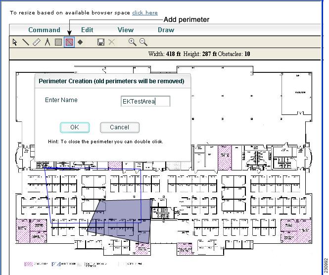
Step 5 ![]() At the Map Editor screen, click the Add Perimeter icon on the tool bar (see Figure 5-1).
At the Map Editor screen, click the Add Perimeter icon on the tool bar (see Figure 5-1).
A pop-up window appears.
Note ![]() An example of a polygon-shaped area is seen in Figure 5-1.
An example of a polygon-shaped area is seen in Figure 5-1.
Figure 5-1 Map Editor Page
Step 6 ![]() Enter the name of the area that you are defining. Click OK.
Enter the name of the area that you are defining. Click OK.
A drawing tool appears.
Step 7 ![]() Move the drawing tool to the area you want to outline.
Move the drawing tool to the area you want to outline.
•![]() Click the left mouse button to begin and end drawing a line.
Click the left mouse button to begin and end drawing a line.
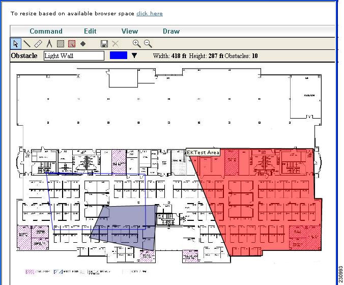
•![]() When you have completely outlined the area, double click the left mouse button and the area is highlighted on the screen (see Figure 5-2).
When you have completely outlined the area, double click the left mouse button and the area is highlighted on the screen (see Figure 5-2).
•![]() The outlined area must be a closed object to highlight on the map.
The outlined area must be a closed object to highlight on the map.
Figure 5-2 Polygon Area
Step 8 ![]() Click the disk icon in the tool bar to save the newly drawn area.
Click the disk icon in the tool bar to save the newly drawn area.
Step 9 ![]() Choose Command > Exit to close the window. You are returned to the original floor plan.
Choose Command > Exit to close the window. You are returned to the original floor plan.
Note ![]() When you return to the original floor plan view, after exiting the map editor, the newly drawn area is not seen; however, it appears in the Planning Model window when you add elements.
When you return to the original floor plan view, after exiting the map editor, the newly drawn area is not seen; however, it appears in the Planning Model window when you add elements.
Step 10 ![]() Select Planning Model from the Select a command drop-down menu to begin adding elements to the newly defined polygon-shaped area.
Select Planning Model from the Select a command drop-down menu to begin adding elements to the newly defined polygon-shaped area.
Using Planning Mode to Calculate Access Point Requirements
The WCS planning mode enables you to calculate the number of access points required to cover an area by placing fictitious access points on a map and allowing you to view the coverage area. Based on the throughput specified for each protocol (802.11a/n or 802.11b/g/n), planning mode calculates the total number of access points required to provide optimum coverage in your network. You can calculate the recommended number and location of access points based on the following criteria:
•![]() traffic type active on the network: data or voice traffic or both
traffic type active on the network: data or voice traffic or both
•![]() location accuracy requirements
location accuracy requirements
•![]() number of active users
number of active users
•![]() number of users per square footage
number of users per square footage
To calculate the recommended number and placement of access points for a given deployment, follow these steps:
Step 1 ![]() Choose Monitor > Maps.
Choose Monitor > Maps.
The window appears (see Figure 5-3).
Figure 5-3 Monitor > Maps Page

Step 2 ![]() Click the appropriate location link from the list that appears.
Click the appropriate location link from the list that appears.
A color-coded map appears showing placement of all installed elements (access points, clients, tags) and their relative signal strength (see Figure 5-4).
Figure 5-4 Selected Floor Area Showing Current Access Point Assignments
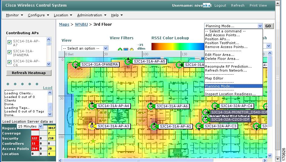
Step 3 ![]() Choose Planning Mode from the Select a command drop-down menu (top-right) and click GO. A blank floor map appears.
Choose Planning Mode from the Select a command drop-down menu (top-right) and click GO. A blank floor map appears.
Step 4 ![]() Click Add APs.
Click Add APs.
Step 5 ![]() In the page that appears, drag the dashed-line rectangle over the map location for which you want to calculate the recommended access points (see Figure 5-5).
In the page that appears, drag the dashed-line rectangle over the map location for which you want to calculate the recommended access points (see Figure 5-5).
Note ![]() Adjust the size or placement of the rectangle by selecting the edge of the rectangle and holding down the Ctrl key. Move the mouse as necessary to outline the targeted location.
Adjust the size or placement of the rectangle by selecting the edge of the rectangle and holding down the Ctrl key. Move the mouse as necessary to outline the targeted location.
Figure 5-5 Add APs Page
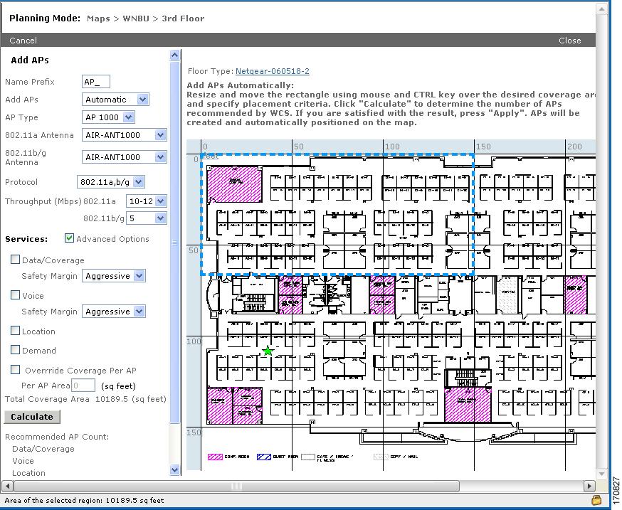
Step 6 ![]() Select Automatic from the Add APs drop-down menu.
Select Automatic from the Add APs drop-down menu.
Step 7 ![]() Select the AP Type and the appropriate antenna and protocol for that access point.
Select the AP Type and the appropriate antenna and protocol for that access point.
Step 8 ![]() Select the target throughput for the access point.
Select the target throughput for the access point.
Step 9 ![]() Check the box(es) next to the service(s) that will be used on the floor. Options are Data/Coverage (default), Voice, and Location (Table 5-2).
Check the box(es) next to the service(s) that will be used on the floor. Options are Data/Coverage (default), Voice, and Location (Table 5-2).
Note ![]() You must select at least one service or an error occurs.
You must select at least one service or an error occurs.
Note ![]() If you check the Advanced Options box, two additional access point planning options appear: Demand and Override Coverage per AP. Additionally, a Safety Margin parameter appears for the Data/Coverage and Voice service options (Table 5-3).
If you check the Advanced Options box, two additional access point planning options appear: Demand and Override Coverage per AP. Additionally, a Safety Margin parameter appears for the Data/Coverage and Voice service options (Table 5-3).
Table 5-2 Definition of Service Options
Table 5-3 Definition of Advanced Options
Step 10 ![]() Click Calculate.
Click Calculate.
The recommended number of access points given the selected services appears (see Figure 5-6).
Figure 5-6 Recommended Number of Access Points Given Selected Services and Parameters
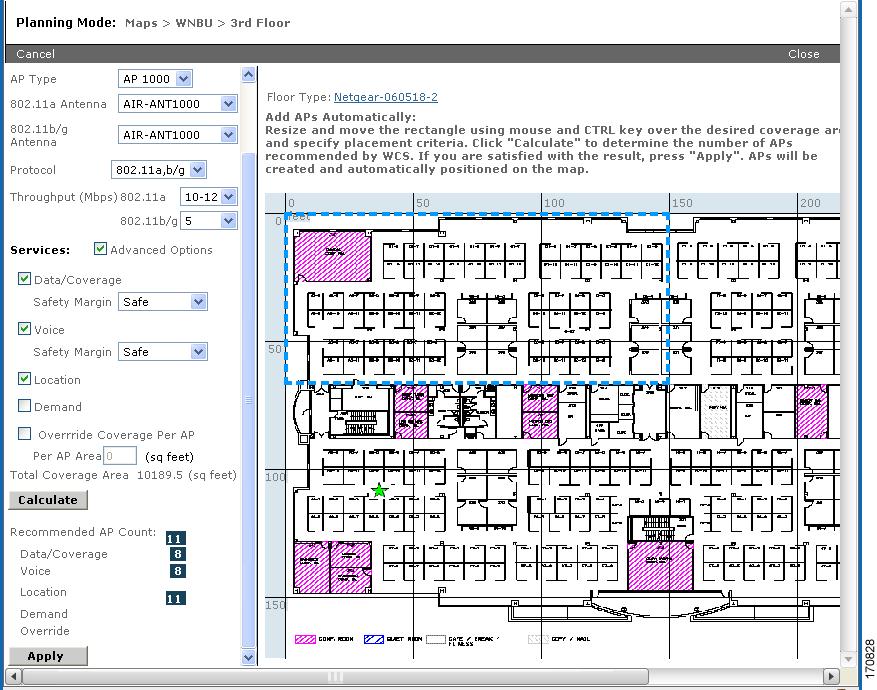
Note ![]() Recommended calculations assume the need for consistently strong signals unless adjusted downward by the safety margin advanced option. In some cases, the recommended number of access points is higher than what is required.
Recommended calculations assume the need for consistently strong signals unless adjusted downward by the safety margin advanced option. In some cases, the recommended number of access points is higher than what is required.
Note ![]() Walls are not used or accounted for in planning mode calculations.
Walls are not used or accounted for in planning mode calculations.
Step 11 ![]() Click Apply to generate a map that shows proposed deployment of the recommended access points in the selected area based on the selected services and parameters.
Click Apply to generate a map that shows proposed deployment of the recommended access points in the selected area based on the selected services and parameters.
Figure 5-7 Recommended Access Point Deployment Given Selected Services and Parameters
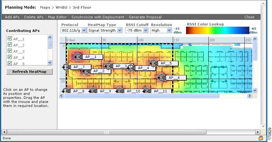
Step 12 ![]() Choose Generate Proposal to display a textual and graphical report of the recommended access point number and deployment based on the given input.
Choose Generate Proposal to display a textual and graphical report of the recommended access point number and deployment based on the given input.
Inspect Location Readiness
The Inspect Location Readiness feature is a distance-based predictive tool that can point out problem areas with access point placement.
The Inspect Location Readiness tool:
•![]() Displays areas that have the required access point coverage and will provide accurate location results.
Displays areas that have the required access point coverage and will provide accurate location results.
•![]() Takes into consideration the placement of each access point along with the inter-access point spacing.
Takes into consideration the placement of each access point along with the inter-access point spacing.
•![]() Assumes that access points and controllers are known to WCS.
Assumes that access points and controllers are known to WCS.
A point is defined as "location-ready" if the following is true:
•![]() At least four access points are deployed on the floor.
At least four access points are deployed on the floor.
•![]() At least three access points are within 70 feet of the point-in-question.
At least three access points are within 70 feet of the point-in-question.
•![]() At least one access point is found to be resident in each quadrant surrounding the point-in-question.
At least one access point is found to be resident in each quadrant surrounding the point-in-question.
To access the Inspect Location Readiness tool, follow these steps:
Step 1 ![]() Choose Monitor > Maps.
Choose Monitor > Maps.
Step 2 ![]() Choose the applicable floor area name.
Choose the applicable floor area name.
Step 3 ![]() From the Select a command drop-down menu, click Inspect Location Readiness.
From the Select a command drop-down menu, click Inspect Location Readiness.
Inspect VoWLAN Readiness
Voice readiness tool (the VoWLAN Readiness tool) allows you to verify that the RF coverage is sufficient for your voice needs. This tool verifies RSSI levels after access points have been installed.
To access the VoWLAN Readiness Tool (VRT), follow these steps:
Step 1 ![]() Choose Monitor > Maps.
Choose Monitor > Maps.
Step 2 ![]() Choose the applicable floor area name.
Choose the applicable floor area name.
Step 3 ![]() From the Select a command drop-down menu, click Inspect VoWLAN Readiness.
From the Select a command drop-down menu, click Inspect VoWLAN Readiness.
Step 4 ![]() Choose the applicable Band, AP Transmit Power, and Client parameters from the drop-down menus.
Choose the applicable Band, AP Transmit Power, and Client parameters from the drop-down menus.
Note ![]() By default, the region map displays the region map for the b/g/n band for Cisco phone based RSSI threshold. The new settings cannot be saved.
By default, the region map displays the region map for the b/g/n band for Cisco phone based RSSI threshold. The new settings cannot be saved.
Step 5 ![]() Depending on the selected client, the RSSI values may not be editable.
Depending on the selected client, the RSSI values may not be editable.
•![]() Cisco Phone—RSSI values are not editable.
Cisco Phone—RSSI values are not editable.
•![]() Custom—RSSI values are editable with the following ranges:
Custom—RSSI values are editable with the following ranges:
–![]() Low threshold between -95dBm to -45dBm
Low threshold between -95dBm to -45dBm
–![]() High threshold between -90dBm to -40dBm
High threshold between -90dBm to -40dBm
Step 6 ![]() The following color schemes indicate whether or not the area is Voice Ready:
The following color schemes indicate whether or not the area is Voice Ready:
•![]() Green—Yes
Green—Yes
•![]() Yellow—Marginal
Yellow—Marginal
•![]() Red—No
Red—No
Troubleshooting Voice RF Coverage Issues
Perform the following to troubleshoot voice RF coverage issues:
•![]() Set the AP Transmit parameter to Max (the maximum downlink power setting). If the map still shows some yellow or red regions, more access points are required to cover the floor.
Set the AP Transmit parameter to Max (the maximum downlink power setting). If the map still shows some yellow or red regions, more access points are required to cover the floor.
•![]() Increase the power level of the access points if a calibrated model shows red or yellow regions (where voice is expected to be deployed) while the AP Transmit parameter is set to Current.
Increase the power level of the access points if a calibrated model shows red or yellow regions (where voice is expected to be deployed) while the AP Transmit parameter is set to Current.
•![]() Verify the green, yellow, and red regions of the RF environment. These indicators are accurate whether the floor is calibrated or not, but floor calibration improves the accuracy.
Verify the green, yellow, and red regions of the RF environment. These indicators are accurate whether the floor is calibrated or not, but floor calibration improves the accuracy.
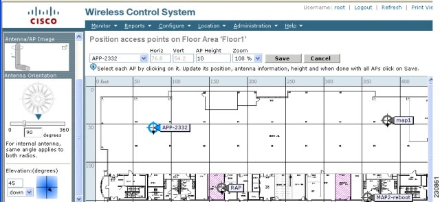
Adding Access Points
After you add the .PNG, .JPG, .JPEG, or .GIF format floor plan and outdoor area maps to the Cisco WCS database, you can position lightweight access point icons on the maps to show where they are installed in the buildings. Follow these steps to add access points to floor plan and outdoor area maps.
Step 1 ![]() Click the desired floor plan or outdoor area map in the Coverage Areas component of the General tab. WCS displays the associated coverage area map.
Click the desired floor plan or outdoor area map in the Coverage Areas component of the General tab. WCS displays the associated coverage area map.
Step 2 ![]() From the Select a command drop-down menu, choose Add Access Points and click GO.
From the Select a command drop-down menu, choose Add Access Points and click GO.
Step 3 ![]() On the Add Access Points page, choose the access points to add to the map.
On the Add Access Points page, choose the access points to add to the map.
Step 4 ![]() Click OK to add the access points to the map and display the Position Access Points map.
Click OK to add the access points to the map and display the Position Access Points map.
Note ![]() The access point icons appear in the upper left area of the map.
The access point icons appear in the upper left area of the map.
Step 5 ![]() Click and drag the icons to indicate their physical locations.
Click and drag the icons to indicate their physical locations.
Step 6 ![]() Click each icon and choose the antenna orientation in the sidebar (see Figure 5-8).
Click each icon and choose the antenna orientation in the sidebar (see Figure 5-8).
Figure 5-8 Antenna Sidebar
Note![]() •
•![]() The antenna angle is relative to the map's X axis. Because the origin of the X (horizontal) and Y (vertical) axes is in the upper left corner of the map, 0 degrees points side A of the access point to the right, 90 degrees points side A down, 180 degrees points side A to the left, and so on.
The antenna angle is relative to the map's X axis. Because the origin of the X (horizontal) and Y (vertical) axes is in the upper left corner of the map, 0 degrees points side A of the access point to the right, 90 degrees points side A down, 180 degrees points side A to the left, and so on.
•![]() The antenna elevation is used to move the antenna vertically, up or down, to a maximum of 90 degrees.
The antenna elevation is used to move the antenna vertically, up or down, to a maximum of 90 degrees.
•![]() Make sure each access point is in the correct location on the map and has the correct antenna orientation. Accurate access point positioning is critical when you use the maps to find coverage holes and rogue access points.
Make sure each access point is in the correct location on the map and has the correct antenna orientation. Accurate access point positioning is critical when you use the maps to find coverage holes and rogue access points.
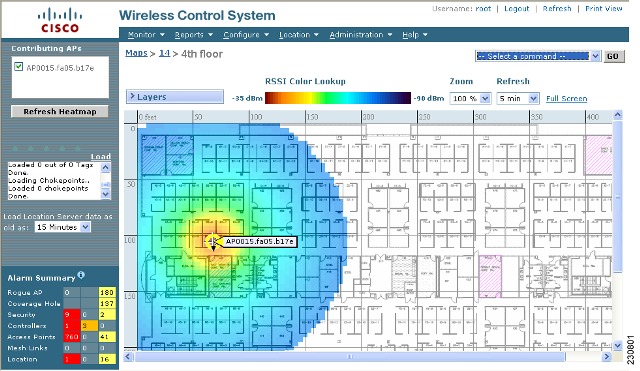
Step 7 ![]() Click Save to store the access point locations and orientations. WCS computes the RF prediction for the coverage area. These RF predictions are popularly known as heat maps because they show the relative intensity of the RF signals on the coverage area map. Figure 5-9 shows an RF prediction heat map.
Click Save to store the access point locations and orientations. WCS computes the RF prediction for the coverage area. These RF predictions are popularly known as heat maps because they show the relative intensity of the RF signals on the coverage area map. Figure 5-9 shows an RF prediction heat map.
Note ![]() This display is only an approximation of the actual RF signal intensity because it does not take into account the attenuation of various building materials, such as drywall or metal objects, nor does it display the effects of RF signals bouncing off obstructions.
This display is only an approximation of the actual RF signal intensity because it does not take into account the attenuation of various building materials, such as drywall or metal objects, nor does it display the effects of RF signals bouncing off obstructions.
Figure 5-9 RF Prediction Heat Map
Access Point Placement
To determine the optimum location of all devices in the wireless LAN coverage areas, you need to consider the access point density and location.
Ensure that no fewer than 3 access points, and preferably 4 or 5, provide coverage to every area where device location is required. The more access points that detect a device, the better. This high level guideline translates into the following best practices, ordered by priority:
1. ![]() Most importantly, access points should surround the desired location.
Most importantly, access points should surround the desired location.
2. ![]() One access point should be placed roughly every 50 to 70 linear feet ( about 17 to 20 meters). This translates into one access point every 2,500 to 5000 square feet (about 230 to 450 square meters).
One access point should be placed roughly every 50 to 70 linear feet ( about 17 to 20 meters). This translates into one access point every 2,500 to 5000 square feet (about 230 to 450 square meters).
Note ![]() The access point must be mounted so that it is under 20 feet high. For best performance, a mounting at 10 feet would be ideal.
The access point must be mounted so that it is under 20 feet high. For best performance, a mounting at 10 feet would be ideal.
Following these guidelines makes it more likely that access points will detect tracked devices. Rarely do two physical environments have the same RF characteristics. Users may need to adjust those parameters to their specific environment and requirements.
Note ![]() Devices must be detected at signals greater than -75 dBm for the controllers to forward information to the location appliance. No fewer than three access points should be able to detect any device at signals below -75 dBm.
Devices must be detected at signals greater than -75 dBm for the controllers to forward information to the location appliance. No fewer than three access points should be able to detect any device at signals below -75 dBm.
Guidelines for Placing Access Points
Follow these rules for placing access points accurately:
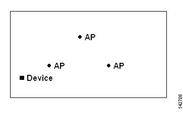
1. ![]() Place access points along the periphery of coverage areas in order to keep devices close to the exterior of rooms and buildings (see Figure 5-10). Access points placed in the center of these coverage areas provide good data on devices that would otherwise appear equidistant from all other access points.
Place access points along the periphery of coverage areas in order to keep devices close to the exterior of rooms and buildings (see Figure 5-10). Access points placed in the center of these coverage areas provide good data on devices that would otherwise appear equidistant from all other access points.
Figure 5-10 Access Points Clustered Together
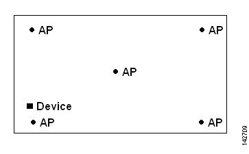
2. ![]() By increasing overall access point density and moving access points towards the perimeter of the coverage area, location accuracy is greatly improved (see Figure 5-11).
By increasing overall access point density and moving access points towards the perimeter of the coverage area, location accuracy is greatly improved (see Figure 5-11).
Figure 5-11 Improved Location Accuracy by Increasing Density
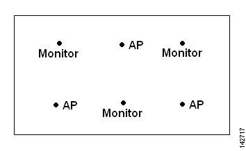
3. ![]() In long and narrow coverage areas, avoid placing access points in a straight line (see Figure 5-12). Stagger them so that each access point is more likely to provide a unique snapshot of a device's location.
In long and narrow coverage areas, avoid placing access points in a straight line (see Figure 5-12). Stagger them so that each access point is more likely to provide a unique snapshot of a device's location.
Figure 5-12 Refrain From Straight Line Placement
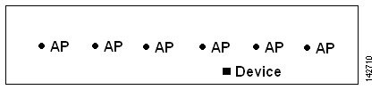
Although the design in Figure 5-12 may provide enough access point density for high bandwidth applications, location suffers because each access point's view of a single device is not varied enough; therefore, location is difficult to determine.
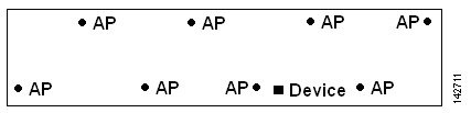
4. ![]() Move the access points to the perimeter of the coverage area and stagger them. Each has a greater likelihood of offering a distinctly different view of the device, resulting in higher location accuracy (see Figure 5-13).
Move the access points to the perimeter of the coverage area and stagger them. Each has a greater likelihood of offering a distinctly different view of the device, resulting in higher location accuracy (see Figure 5-13).
Figure 5-13 Improved Location Accuracy by Staggering Around Perimeter
5. ![]() Designing a location-aware wireless LAN, while planning for voice as well, is better done with a few things in mind. Most current wireless handsets support only 802.11b/n, which offers only three non-overlapping channels. Therefore, wireless LANs designed for telephony tend to be less dense than those planned to carry data. Also, when traffic is queued in the Platinum QoS bucket (typically reserved for voice and other latency-sensitive traffic), lightweight access points postpone their scanning functions that allow them to peak at other channels and collect, among other things, device location information. The user has the option to supplement the wireless LAN deployment with access points set to monitor-only mode. Access points that perform only monitoring functions do not provide service to clients and do not create any interference. They simply scan the airwaves for device information.
Designing a location-aware wireless LAN, while planning for voice as well, is better done with a few things in mind. Most current wireless handsets support only 802.11b/n, which offers only three non-overlapping channels. Therefore, wireless LANs designed for telephony tend to be less dense than those planned to carry data. Also, when traffic is queued in the Platinum QoS bucket (typically reserved for voice and other latency-sensitive traffic), lightweight access points postpone their scanning functions that allow them to peak at other channels and collect, among other things, device location information. The user has the option to supplement the wireless LAN deployment with access points set to monitor-only mode. Access points that perform only monitoring functions do not provide service to clients and do not create any interference. They simply scan the airwaves for device information.
Less dense wireless LAN installations, such as voice networks, find their location accuracy greatly increased by the addition and proper placement of monitor access points (see Figure 5-14).
Figure 5-14 Less Dense Wireless LAN Installations
6. ![]() Verify coverage using a wireless laptop, handheld, or phone to ensure that no fewer than three access points are detected by the device. To verify client and asset tag location, ensure that WCS reports client devices and tags within the specified accuracy range (10 m, 90%).
Verify coverage using a wireless laptop, handheld, or phone to ensure that no fewer than three access points are detected by the device. To verify client and asset tag location, ensure that WCS reports client devices and tags within the specified accuracy range (10 m, 90%).
Creating a Network Design
After access points have been installed and have joined a controller, and WCS has been configured to manage the controllers, set up a network design. A network design is a representation within WCS of the physical placement of access points throughout facilities. A hierarchy of a single campus, the buildings that comprise that campus, and the floors of each building constitute a single network design. These steps assume that the location appliance is set to poll the controllers in that network, as well as be configured to synchronize with that specific network design, in order to track devices in that environment. The concept and steps to perform synchronization between WCS and the location appliance are explained in the "Importing the Location Appliance into WCS" section on page 11-8.
Designing a Network
Follow these steps to design a network.
Step 1 ![]() Open the WCS web interface and log in.
Open the WCS web interface and log in.
Note ![]() To create or edit a network design, you must log into WCS and have SuperUser, Admin, or ConfigManager access privileges.
To create or edit a network design, you must log into WCS and have SuperUser, Admin, or ConfigManager access privileges.
Step 2 ![]() Click the Monitor tab and choose the Maps subtab (see Figure 5-15).
Click the Monitor tab and choose the Maps subtab (see Figure 5-15).
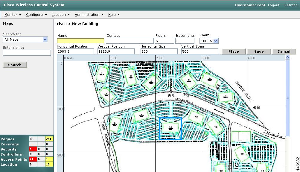
Step 3 ![]() From the drop-down menu on the right-hand side, choose either New Campus or New Building, depending on the size of the network design and the organization of maps. If you chose New Campus, continue to Step 4. To create a building without a campus, skip to Step 13.
From the drop-down menu on the right-hand side, choose either New Campus or New Building, depending on the size of the network design and the organization of maps. If you chose New Campus, continue to Step 4. To create a building without a campus, skip to Step 13.
Figure 5-15 Creating a New Network Design
Step 4 ![]() Click GO.
Click GO.
Step 5 ![]() Enter a name for the campus network design, a contact name, and the file path to the campus image file. .bmps and .jgps are importable.
Enter a name for the campus network design, a contact name, and the file path to the campus image file. .bmps and .jgps are importable.
Step 6 ![]() Check the Maintain Aspect Ratio check box. Enabling this check box causes the horizontal span of the campus to be 5000 feet and adjusts the vertical span according to the image file's aspect ratio. Adjusting either the horizontal or vertical span changes the other field in accordance with the image ratio.
Check the Maintain Aspect Ratio check box. Enabling this check box causes the horizontal span of the campus to be 5000 feet and adjusts the vertical span according to the image file's aspect ratio. Adjusting either the horizontal or vertical span changes the other field in accordance with the image ratio.
You should uncheck the Maintain Aspect Ratio check box if you want to override this automatic adjustment. You could then adjust both span values to match the real world campus dimensions.
Step 7 ![]() Click OK.
Click OK.
Step 8 ![]() On the Monitor > Maps subtab, click the hyperlink associated with the above-made campus map. A window showing the new campus image is displayed.
On the Monitor > Maps subtab, click the hyperlink associated with the above-made campus map. A window showing the new campus image is displayed.
Step 9 ![]() From the drop-down menu on the upper right of the window, select New Building and click GO (see Figure 5-16).
From the drop-down menu on the upper right of the window, select New Building and click GO (see Figure 5-16).
Figure 5-16 New Building
Step 10 ![]() Enter the name of the building, the contact person, and the number of floors and basements in the building.
Enter the name of the building, the contact person, and the number of floors and basements in the building.
Step 11 ![]() Indicate which building on the campus map is the correct building by clicking the blue box in the upper left of the campus image and dragging it to the intended location (see Figure 5-17). To resize the blue box, hold down the Ctrl key and click and drag to adjust its horizontal size. You can also enter dimensions of the building by entering numerical values in the Horizontal Span and Vertical Span fields and click Place. After resizing, reposition the blue box if necessary by clicking on it and dragging it to the desired location. Click Save.
Indicate which building on the campus map is the correct building by clicking the blue box in the upper left of the campus image and dragging it to the intended location (see Figure 5-17). To resize the blue box, hold down the Ctrl key and click and drag to adjust its horizontal size. You can also enter dimensions of the building by entering numerical values in the Horizontal Span and Vertical Span fields and click Place. After resizing, reposition the blue box if necessary by clicking on it and dragging it to the desired location. Click Save.
Figure 5-17 Repositioning Building Highlighted in Blue
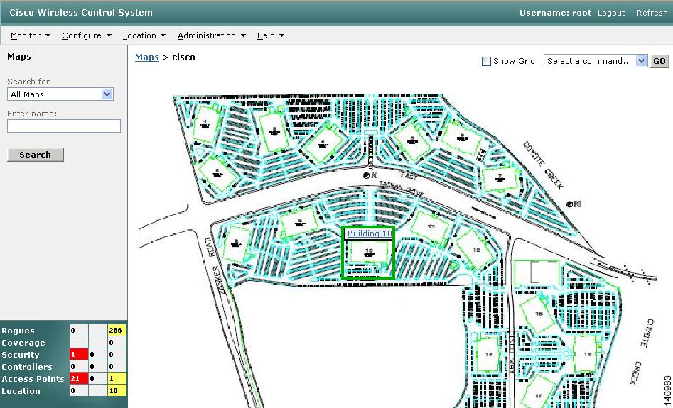
Step 12 ![]() WCS is then returned to the campus image with the newly created building highlighted in a green box. Click the green box (see Figure 5-18).
WCS is then returned to the campus image with the newly created building highlighted in a green box. Click the green box (see Figure 5-18).
Figure 5-18 Newly Created Building Highlighted in Green
Step 13 ![]() To create a building without a campus, choose New Building and click GO.
To create a building without a campus, choose New Building and click GO.
Step 14 ![]() Enter the building's name, contact information, number of floors and basements, and dimension information. Click Save. WCS is returned to the Monitor > Maps window.
Enter the building's name, contact information, number of floors and basements, and dimension information. Click Save. WCS is returned to the Monitor > Maps window.
Step 15 ![]() Click the hyperlink associated with the newly created building.
Click the hyperlink associated with the newly created building.
Step 16 ![]() On the Monitor > Maps > [Campus Name] > [Building Name] window, go to the drop-down menu and choose New Floor Area. Click GO.
On the Monitor > Maps > [Campus Name] > [Building Name] window, go to the drop-down menu and choose New Floor Area. Click GO.
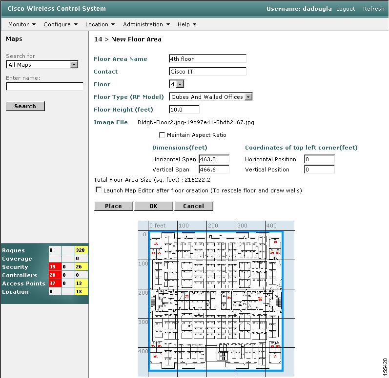
Step 17 ![]() Enter a name for the floor, a contact, a floor number, floor type, and height at which the access points are installed and the path of the floor image. Click Next.
Enter a name for the floor, a contact, a floor number, floor type, and height at which the access points are installed and the path of the floor image. Click Next.
Note ![]() The Floor Type (RF Model) field specifies the type of environment on that specific floor. This RF Model indicates the amount of RF signal attenuation likely to be present on that floor. If the available models do not properly characterize a floor's makeup, details on how to create RF models specific to a floor's attenuation characteristics are available in the "Creating and Applying Calibration Models" section.
The Floor Type (RF Model) field specifies the type of environment on that specific floor. This RF Model indicates the amount of RF signal attenuation likely to be present on that floor. If the available models do not properly characterize a floor's makeup, details on how to create RF models specific to a floor's attenuation characteristics are available in the "Creating and Applying Calibration Models" section.
Step 18 ![]() If the floor area is a different dimension than the building, adjust floor dimensions by either making numerical changes to the text fields under the Dimensions heading or by holding the Ctrl key and clicking and dragging the blue box around the floor image. If the floor's location is offset from the upper left corner of the building, change the placement of the floor within the building by either clicking and dragging the blue box to the desired location or by altering the numerical values under the Coordinates of top left corner heading (see Figure 5-19). After making changes to any numerical values, click Place.
If the floor area is a different dimension than the building, adjust floor dimensions by either making numerical changes to the text fields under the Dimensions heading or by holding the Ctrl key and clicking and dragging the blue box around the floor image. If the floor's location is offset from the upper left corner of the building, change the placement of the floor within the building by either clicking and dragging the blue box to the desired location or by altering the numerical values under the Coordinates of top left corner heading (see Figure 5-19). After making changes to any numerical values, click Place.
Figure 5-19 Repositioning Using Numerical Value Fields
Step 19 ![]() Adjust the floor's characteristics with the WCS map editor by choosing the check box next to Launch Map Editor. For an explanation of the map editor feature, see the "Using the Map Editor to Enhance Floor Plans" section.
Adjust the floor's characteristics with the WCS map editor by choosing the check box next to Launch Map Editor. For an explanation of the map editor feature, see the "Using the Map Editor to Enhance Floor Plans" section.
Step 20 ![]() At the new floor's image window (Monitor > Maps > [CampusName] > [BuildingName] > [FloorName]), go to the drop-down menu on the upper right and choose Add Access Points. Click GO.
At the new floor's image window (Monitor > Maps > [CampusName] > [BuildingName] > [FloorName]), go to the drop-down menu on the upper right and choose Add Access Points. Click GO.
Step 21 ![]() All access points that are connected to controllers are displayed. Even controllers that WCS is configured to manage but which have not yet been added to another floor map are displayed. Select the access points to be placed on the specific floor map by checking the boxes to the left of the access point entries. Check the box to the left of the Name column to select all access points. Click OK.
All access points that are connected to controllers are displayed. Even controllers that WCS is configured to manage but which have not yet been added to another floor map are displayed. Select the access points to be placed on the specific floor map by checking the boxes to the left of the access point entries. Check the box to the left of the Name column to select all access points. Click OK.
Step 22 ![]() Each access point you have chosen to add to the floor map is represented by a gray circle (differentiated by access point name or MAC address) and is lined up in the upper left part of the floor map. Drag each access point to the appropriate location. (Access points turn blue when you click on them to relocate them.) The small black arrow at the side of each access point represents Side A of each access point, and each access point's arrow must correspond with the direction in which the access points were installed. (Side A is clearly noted on each 1000 series access point and has no relevance to the 802.11a/n radio.)
Each access point you have chosen to add to the floor map is represented by a gray circle (differentiated by access point name or MAC address) and is lined up in the upper left part of the floor map. Drag each access point to the appropriate location. (Access points turn blue when you click on them to relocate them.) The small black arrow at the side of each access point represents Side A of each access point, and each access point's arrow must correspond with the direction in which the access points were installed. (Side A is clearly noted on each 1000 series access point and has no relevance to the 802.11a/n radio.)
Step 23 ![]() To adjust the directional arrow, choose the appropriate orientation in the Antenna Angle drop-down menu. Click Save when you are finished placing and adjusting each access point's direction.
To adjust the directional arrow, choose the appropriate orientation in the Antenna Angle drop-down menu. Click Save when you are finished placing and adjusting each access point's direction.
Note ![]() Access point placement and direction must directly reflect the actual access point deployment or the system cannot pinpoint the device location.
Access point placement and direction must directly reflect the actual access point deployment or the system cannot pinpoint the device location.
Step 24 ![]() Repeat the above processes to create campuses, buildings, and floors until each device location is properly detailed in a network design.
Repeat the above processes to create campuses, buildings, and floors until each device location is properly detailed in a network design.
Changing Access Point Positions by Importing and Exporting a File
You can change an access point position by importing or exporting a file. The file contains only the lines describing the access point you want to move. This option takes less time than manually changing multiple access point positions. Follow these steps to change access point positions using the importing or exporting of a file.
Step 1 ![]() Choose Monitor > Maps.
Choose Monitor > Maps.
Step 2 ![]() From the Select a command drop-down menu, choose Properties.
From the Select a command drop-down menu, choose Properties.
Step 3 ![]() At the Unit of Dimension drop-down menu, choose feet or meters.
At the Unit of Dimension drop-down menu, choose feet or meters.
Step 4 ![]() The Advanced Debug option must be enabled on both the location appliance and WCS so the location accuracy testpoint is correct.
The Advanced Debug option must be enabled on both the location appliance and WCS so the location accuracy testpoint is correct.
Step 5 ![]() In the Import/Export AP Placement portion of the window, click Browse to find the file you want to import. The file in the [BuildingName], [FloorName], [APName], (aAngle), (bAngle), [X], [Y], ([aAngleElevation, bAngleElevation, Z]), (aAntennaType, aAntennaMode, (aAntennaPattern, (aAntennaGain)), bAntennaType, bAntennaDiversity, (bAntennaPattern, bAntennaGain))))) format must have already been created and added to WCS. (Refer to the "Inspect VoWLAN Readiness" section.)
In the Import/Export AP Placement portion of the window, click Browse to find the file you want to import. The file in the [BuildingName], [FloorName], [APName], (aAngle), (bAngle), [X], [Y], ([aAngleElevation, bAngleElevation, Z]), (aAntennaType, aAntennaMode, (aAntennaPattern, (aAntennaGain)), bAntennaType, bAntennaDiversity, (bAntennaPattern, bAntennaGain))))) format must have already been created and added to WCS. (Refer to the "Inspect VoWLAN Readiness" section.)
Note ![]() The parameters in square brackets are mandatory, and those in parentheses are optional.
The parameters in square brackets are mandatory, and those in parentheses are optional.
Note ![]() Angles must be entered in radians (X,Y), and the height is entered in feet. The aAngle and bAngle range is from -2Pi (-6.28...) to 2Pi (6.28...), and the elevation ranges from -Pi (-3.14..) to Pi (3.14..).
Angles must be entered in radians (X,Y), and the height is entered in feet. The aAngle and bAngle range is from -2Pi (-6.28...) to 2Pi (6.28...), and the elevation ranges from -Pi (-3.14..) to Pi (3.14..).
Step 6 ![]() Click Import. The RF calculation takes approximately two seconds per access point.
Click Import. The RF calculation takes approximately two seconds per access point.
Using Chokepoints to Enhance Tag Location Reporting
Installation of chokepoints provides enhanced location information for RFID tags. When an active Cisco Compatible Extensions version 1 compliant RFID tag enters the range of a chokepoint, it is stimulated by the chokepoint. The MAC address of this chokepoint is then included in the next beacon sent by the stimulated tag. All access points that detect this tag beacon then forward the information to the controller and location appliance.
Using chokepoints in conjunction with active compatible extensions compliant tags provides immediate location information on a tag and its asset. When a Cisco Compatible Extension's tag moves out of the range of a chokepoint, its subsequent beacon frames do not contain any identifying chokepoint information. Location determination of the tag defaults to the standard calculation methods based on RSSIs reported by the access point associated with the tag.
Adding Chokepoints to the WCS Database and Map
Chokepoints are installed and configured as recommended by the Chokepoint vendor. After the chokepoint installation is complete and operational, the chokepoint is added to WCS and placed on floor maps. They are forwarded to the location server during synchronization.
Follow these steps to add a chokepoint to the WCS database and appropriate map:
Step 1 ![]() Choose Configure > Chokepoints from the main menu.
Choose Configure > Chokepoints from the main menu.
The All Chokepoints summary window appears (see Figure 5-20).
Figure 5-20 Configure > Chokepoints
Step 2 ![]() Select Add Chokepoints from the Select a command menu (Figure 5-20). Click GO.
Select Add Chokepoints from the Select a command menu (Figure 5-20). Click GO.
The Add Chokepoint entry window appears (see Figure 5-21).
Figure 5-21 Add Chokepoint Configuration Page
Step 3 ![]() Enter the MAC address, name, and coverage range for the chokepoint.
Enter the MAC address, name, and coverage range for the chokepoint.
Note ![]() The chokepoint range is product-specific and is supplied by the chokepoint vendor.
The chokepoint range is product-specific and is supplied by the chokepoint vendor.
Step 4 ![]() Specify whether the chokepoint is an entry or exit chokepoint.
Specify whether the chokepoint is an entry or exit chokepoint.
Step 5 ![]() Click OK to save the chokepoint entry to the database.
Click OK to save the chokepoint entry to the database.
The All Chokepoints summary page appears with the new chokepoint entry listed (Figure 5-22).
Figure 5-22 All Chokepoints Summary Page
Note ![]() After the chokepoint is added to the database, place it on the appropriate WCS floor map.
After the chokepoint is added to the database, place it on the appropriate WCS floor map.
Step 6 ![]() To add the chokepoint to a map, choose Monitor > Maps (Figure 5-23).
To add the chokepoint to a map, choose Monitor > Maps (Figure 5-23).
Figure 5-23 Monitor > Maps
Step 7 ![]() On the Maps page, choose the link that corresponds to the floor location of the chokepoint. The floor map appears (Figure 5-24).
On the Maps page, choose the link that corresponds to the floor location of the chokepoint. The floor map appears (Figure 5-24).
Figure 5-24 Selected Floor Map
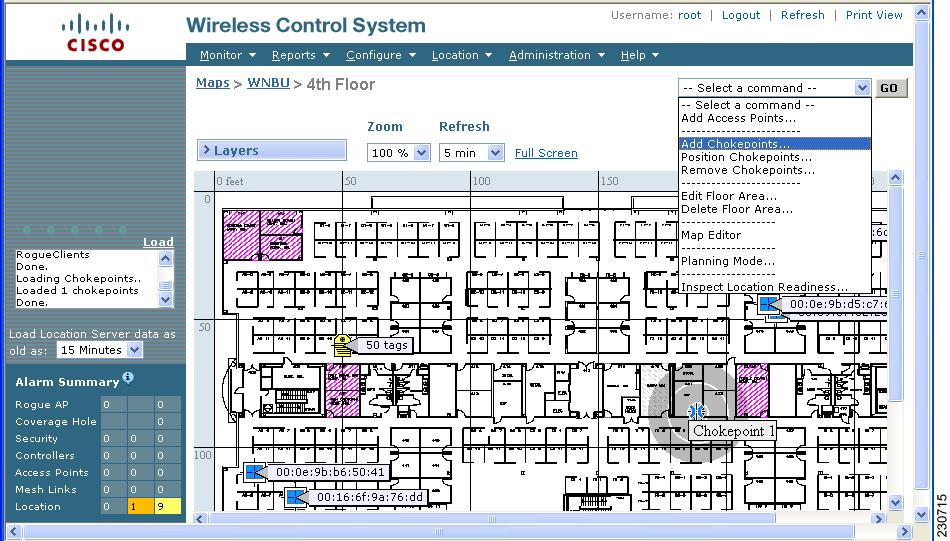
Step 8 ![]() Select Add Chokepoints from the Select a command menu. Click GO.
Select Add Chokepoints from the Select a command menu. Click GO.
The Add Chokepoints summary page appears (see Figure 5-25).
Note ![]() The Add Chokepoints summary page lists all recently-added chokepoints that are in the database but not yet mapped.
The Add Chokepoints summary page lists all recently-added chokepoints that are in the database but not yet mapped.
Figure 5-25 Add Chokepoints Summary Page
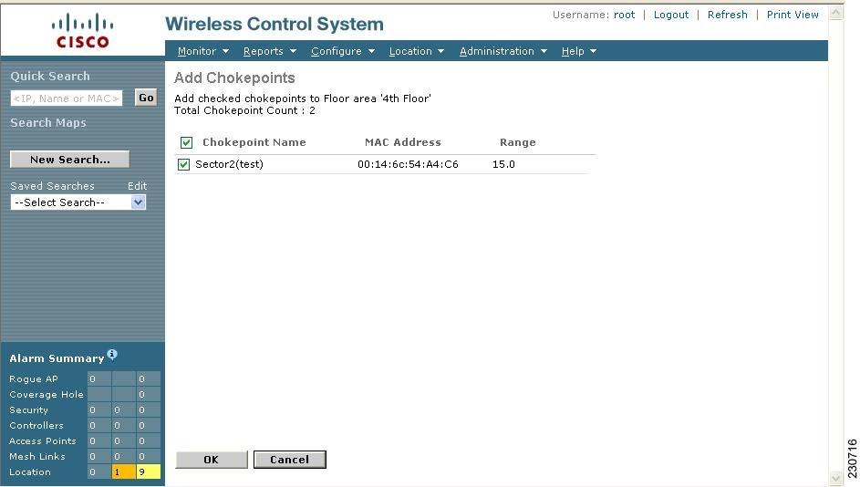
Step 9 ![]() Check the box next to the chokepoint to be added to the map. Click OK.
Check the box next to the chokepoint to be added to the map. Click OK.
A map appears with a chokepoint icon located in the top-left hand corner (Figure 5-26). You are now ready to place the chokepoint on the map.
Figure 5-26 Map for Positioning Chokepoint

Step 10 ![]() Left click on the chokepoint icon and drag and place it in the proper location (see Figure 5-27).
Left click on the chokepoint icon and drag and place it in the proper location (see Figure 5-27).
Figure 5-27 Chokepoint Icon Positioned on the Floor Map
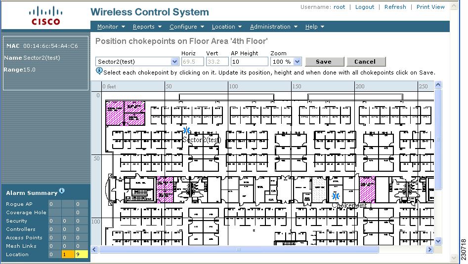
Note ![]() The MAC address, name, and coverage range of the chokepoint appear in the left panel when you click on the chokepoint icon for placement.
The MAC address, name, and coverage range of the chokepoint appear in the left panel when you click on the chokepoint icon for placement.
Step 11 ![]() Click Save when the icon is correctly placed on the map.
Click Save when the icon is correctly placed on the map.
You are returned to the floor map and the added chokepoint appears on the map.
Note ![]() The newly created chokepoint icon may or may not appear on the map depending on the display settings for that floor. If the icon did not appear, proceed with Step 12.
The newly created chokepoint icon may or may not appear on the map depending on the display settings for that floor. If the icon did not appear, proceed with Step 12.
Figure 5-28 New Chokepoint Displays on Floor Map
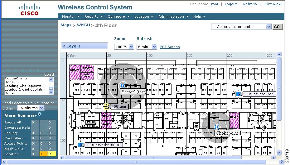
Note ![]() The rings around the chokepoint icon indicate the coverage area. When a Cisco Compatible Extensions tag and its asset passes within the coverage area, location details are broadcast, and the tag is automatically mapped on the chokepoint coverage circle. The chokepoint range is given as a visual only, but chokepoint vendor software is required to actually configure the range. When the tag moves out of the chokepoint range, its location is calculated as before and is no longer mapped on the chokepoint rings. In Figure 5-28, the tag is currently out of range of the chokepoint.
The rings around the chokepoint icon indicate the coverage area. When a Cisco Compatible Extensions tag and its asset passes within the coverage area, location details are broadcast, and the tag is automatically mapped on the chokepoint coverage circle. The chokepoint range is given as a visual only, but chokepoint vendor software is required to actually configure the range. When the tag moves out of the chokepoint range, its location is calculated as before and is no longer mapped on the chokepoint rings. In Figure 5-28, the tag is currently out of range of the chokepoint.
Note ![]() MAC address, name, and range of a chokepoint display when you pass a mouse over its map icon.
MAC address, name, and range of a chokepoint display when you pass a mouse over its map icon.
Step 12 ![]() If the chokepoint does not appear on the map, click Layers to collapse a selection menu of possible elements to display on the map. Click the Chokepoints box.
If the chokepoint does not appear on the map, click Layers to collapse a selection menu of possible elements to display on the map. Click the Chokepoints box.
The chokepoint appears on the map (Figure 5-29).
Figure 5-29 Display Chokepoints on Map
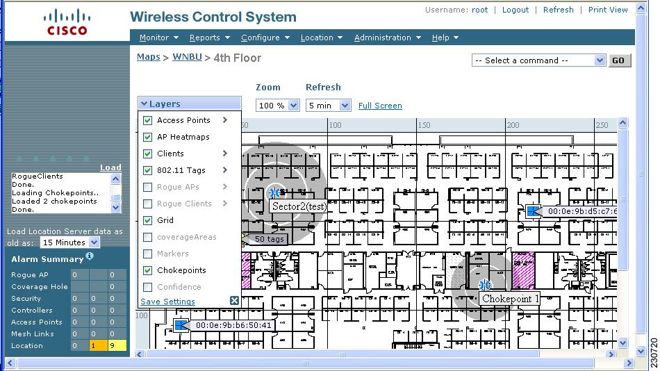
Step 13 ![]() Click X to close the Layers window.
Click X to close the Layers window.
Note ![]() Do not select Save Settings unless you want to save this display criteria for all maps.
Do not select Save Settings unless you want to save this display criteria for all maps.
Removing Chokepoints from the WCS Database and Map
You can remove one or multiple chokepoints at a time.
Follow these steps to delete a chokepoint.
Step 1 ![]() Choose Configure > Chokepoints. The All Chokepoints page appears.
Choose Configure > Chokepoints. The All Chokepoints page appears.
Step 2 ![]() Check the box(es) next to the chokepoint(s) to be deleted.
Check the box(es) next to the chokepoint(s) to be deleted.
Step 3 ![]() Choose Remove Chokepoints from the Select a command drop-down menu. Click GO.
Choose Remove Chokepoints from the Select a command drop-down menu. Click GO.
Step 4 ![]() To confirm chokepoint deletion, click OK in the pop-up window that appears.
To confirm chokepoint deletion, click OK in the pop-up window that appears.
You are returned to the All Chokepoints page. A message confirming deletion of the chokepoint appears. The deleted chokepoint(s) is no longer listed on the page.
Monitoring Chokepoints
Chokepoints are installed and configured as recommended by the chokepoint vendor. Chokepoints are added to WCS and placed on floor maps, and then they are pushed to the location server during synchronization. Choose Monitor > Chokepoints to display a list of found chokepoints. Clicking the link under Map Location for a particular chokepoint displays a map that shows the location of the chokepoint. The following parameters are displayed:
•![]() MAC Address—The MAC address of the chokepoint.
MAC Address—The MAC address of the chokepoint.
•![]() Chokepoint Name—The user-defined name of the chokepoint.
Chokepoint Name—The user-defined name of the chokepoint.
•![]() Entry/Exit Chokepoint—Specifies whether the chokepoint is an entry or exit chokepoint.
Entry/Exit Chokepoint—Specifies whether the chokepoint is an entry or exit chokepoint.
•![]() Range—The range of the chokepoint in feet.
Range—The range of the chokepoint in feet.
•![]() Map Location—A link to a map showing the location of the chokepoint.
Map Location—A link to a map showing the location of the chokepoint.
Monitoring Maps
This section describes how to use maps to monitor your wireless LANs and predict coverage. You can use maps to do the following:
•![]() Monitoring Predicted Coverage
Monitoring Predicted Coverage
•![]() Monitoring Transmit Power Levels on a Floor Map
Monitoring Transmit Power Levels on a Floor Map
•![]() Monitoring Coverage Holes on a Floor Map
Monitoring Coverage Holes on a Floor Map
•![]() Monitoring Clients on a Floor Map
Monitoring Clients on a Floor Map
In preparation for monitoring your wireless LANs, familiar yourself with the various refresh options for a map.
•![]() Refresh from network—By clicking Refresh Heatmap in the left sidebar menu (see callout 1 in Figure 5-30), you can refresh the map status and statistics directly from the controller through an SNMP fetch rather than polled data from the WCS database that is five to fifteen minutes older.
Refresh from network—By clicking Refresh Heatmap in the left sidebar menu (see callout 1 in Figure 5-30), you can refresh the map status and statistics directly from the controller through an SNMP fetch rather than polled data from the WCS database that is five to fifteen minutes older.
Note ![]() If you have monitor mode access points on the floor plan, you have a choice between IDS or coverage heatmap types. A coverage heatmap excludes monitor mode access points, and an IDS heatmap includes them.
If you have monitor mode access points on the floor plan, you have a choice between IDS or coverage heatmap types. A coverage heatmap excludes monitor mode access points, and an IDS heatmap includes them.
•![]() Refresh browser—Above the map next to the Logout and Print option is another refresh option (see callout 3 in Figure 5-30). Clicking this refreshes the complete page, or the map and its status and statistics if you are on a map page.
Refresh browser—Above the map next to the Logout and Print option is another refresh option (see callout 3 in Figure 5-30). Clicking this refreshes the complete page, or the map and its status and statistics if you are on a map page.
•![]() Load—The Load option in the left sidebar menu refreshes map data from the WCS database on demand (see callout 2 in Figure 5-30). Otherwise, the Refresh option (by the Zoom option on the upper right of the map) provides an interval drop-down menu to set how often to refresh the map data from the database.
Load—The Load option in the left sidebar menu refreshes map data from the WCS database on demand (see callout 2 in Figure 5-30). Otherwise, the Refresh option (by the Zoom option on the upper right of the map) provides an interval drop-down menu to set how often to refresh the map data from the database.
Figure 5-30 Monitoring Maps
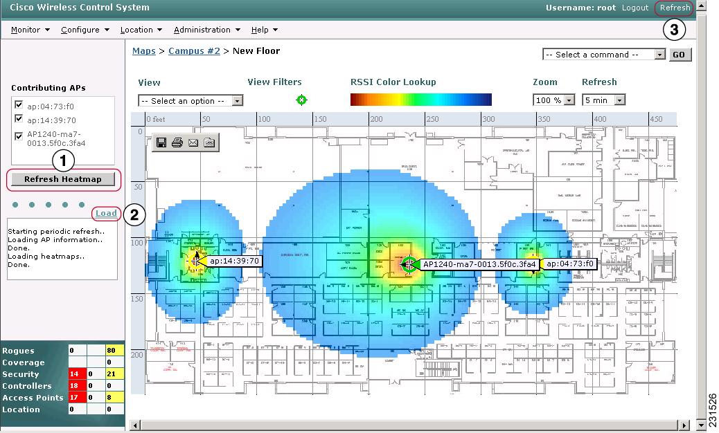
Note ![]() All three options refresh the data based on the layer selection.
All three options refresh the data based on the layer selection.
Monitoring Predicted Coverage
Follow these steps to monitor the predicted wireless LAN coverage on a map.
Step 1 ![]() Click Monitor > Maps to display the Maps page.
Click Monitor > Maps to display the Maps page.
Step 2 ![]() Click an item in the Name column.
Click an item in the Name column.
Step 3 ![]() Click Layers to see a check list of the available layers to view. Choosing some layers results in a popup window to further choose what content gets shown in the map. Those layers with popups are described in the next sections. The layer options are as follows:
Click Layers to see a check list of the available layers to view. Choosing some layers results in a popup window to further choose what content gets shown in the map. Those layers with popups are described in the next sections. The layer options are as follows:
•![]() Access Points
Access Points
•![]() AP Heatmaps
AP Heatmaps
•![]() AP Mesh Info —Displays only if mesh access points are present in outdoor areas.
AP Mesh Info —Displays only if mesh access points are present in outdoor areas.
•![]() Clients —Displays data only if a location server was added in WCS.
Clients —Displays data only if a location server was added in WCS.
•![]() 802.11 Tags
802.11 Tags
•![]() Rogue APs —Displays data only if a location server was added in WCS.
Rogue APs —Displays data only if a location server was added in WCS.
•![]() Rogue Adhocs —Displays data only if a location server was added in WCS.
Rogue Adhocs —Displays data only if a location server was added in WCS.
•![]() Rogue Clients —Displays only if a location server was added in WCS.
Rogue Clients —Displays only if a location server was added in WCS.
•![]() Grid
Grid
•![]() Coverage Areas
Coverage Areas
•![]() Markers
Markers
•![]() Chokepoints — Displays only if chokepoints are added in WCS.
Chokepoints — Displays only if chokepoints are added in WCS.
Note ![]() If you click the arrow to the right of these layers, more filter options are provided.
If you click the arrow to the right of these layers, more filter options are provided.
The enabled layers are checked, and the disabled ones are unavailable.
Note ![]() When you mouse over the various locations, a popup with general, 802.11a/n, and 802.11b/g/n data appears. It provides the channel, transmit power level, user count, utilization count, antenna name, antenna angle, and elevation angle (for the 802.11a/n and 802.11b/g/n windows), and access point MAC address, model, controller IP address, location, and height in the General tab.
When you mouse over the various locations, a popup with general, 802.11a/n, and 802.11b/g/n data appears. It provides the channel, transmit power level, user count, utilization count, antenna name, antenna angle, and elevation angle (for the 802.11a/n and 802.11b/g/n windows), and access point MAC address, model, controller IP address, location, and height in the General tab.
Access Point Layer
If you enable the Access Point layer and then click on the arrow to the right of these layers, anaccess point filter window appears with further menu options (see Figure 5-31).
Figure 5-31 AP Filter Window
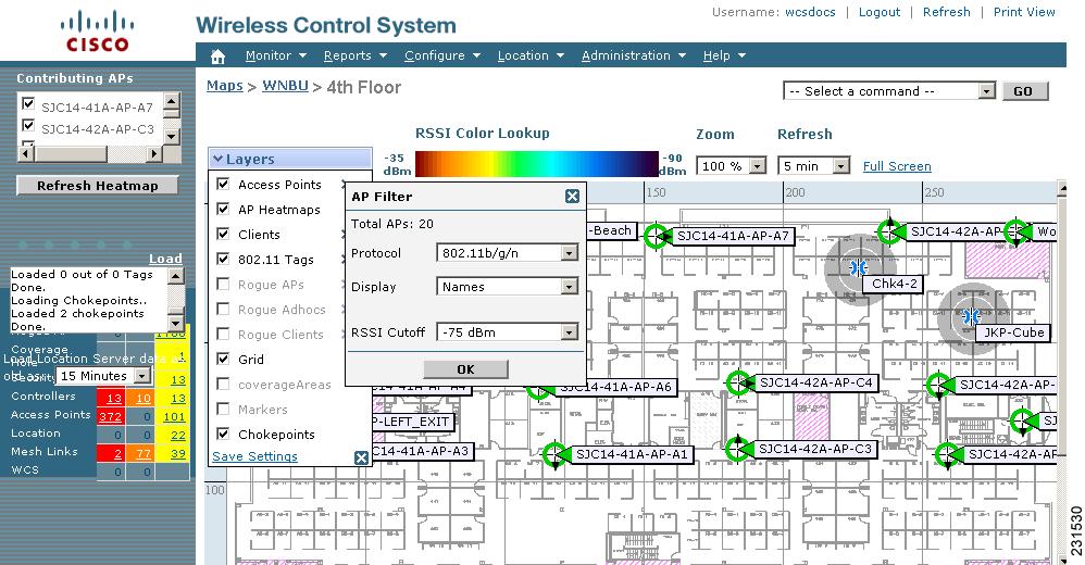
Step 1 ![]() From the Protocol drop-down menu, choose one of the following 802.11 protocols to display on the coverage map:
From the Protocol drop-down menu, choose one of the following 802.11 protocols to display on the coverage map:
•![]() 802.11a/n & b/g/n—Displays all the access points in the area.
802.11a/n & b/g/n—Displays all the access points in the area.
•![]() 802.11a/n—Displays a colored overlay depicting the coverage patterns for the 802.11a/n radios. The colors show the received signal strength from red (-35 dBm) through dark blue (-85 dBm).
802.11a/n—Displays a colored overlay depicting the coverage patterns for the 802.11a/n radios. The colors show the received signal strength from red (-35 dBm) through dark blue (-85 dBm).
•![]() 802.11b/g/n—Displays a colored overlay depicting the coverage patterns for the 802.11b/g/n radios. The colors show the received signal strength from red (-35 dBm) through dark blue (-85 dBm). This is the default value.
802.11b/g/n—Displays a colored overlay depicting the coverage patterns for the 802.11b/g/n radios. The colors show the received signal strength from red (-35 dBm) through dark blue (-85 dBm). This is the default value.
Step 2 ![]() From the Display drop-down menu, choose one of the following options to specify the information that appears in the flag next to each access point on the map:
From the Display drop-down menu, choose one of the following options to specify the information that appears in the flag next to each access point on the map:
•![]() Channels—Shows the Cisco Radio channel number as Ch#nn, where nn is the channel number, or shows Unavailable for unconnected access points.
Channels—Shows the Cisco Radio channel number as Ch#nn, where nn is the channel number, or shows Unavailable for unconnected access points.
•![]() TX Power Level—Shows the current Cisco Radio transmit power level as Tx Power n, where n is power level 1 (high) through 5 (low) or shows Unavailable for unconnected access points.
TX Power Level—Shows the current Cisco Radio transmit power level as Tx Power n, where n is power level 1 (high) through 5 (low) or shows Unavailable for unconnected access points.
•![]() Coverage Holes—Shows the percentage of clients whose signal has become weaker until the client lost its connection, shows Unavailable for unconnected access points, or shows MonitorOnly for access points in Monitor-Only mode.
Coverage Holes—Shows the percentage of clients whose signal has become weaker until the client lost its connection, shows Unavailable for unconnected access points, or shows MonitorOnly for access points in Monitor-Only mode.
•![]() MAC Addresses—Displays the MAC address of the access point, regardless of whether the access point is associated to a controller.
MAC Addresses—Displays the MAC address of the access point, regardless of whether the access point is associated to a controller.
•![]() Names—Displays the access point name. This is the default value.
Names—Displays the access point name. This is the default value.
•![]() Controller IP—Displays the IP address of the controller to which the access point is associated or "Not Associated" for disassociated access points.
Controller IP—Displays the IP address of the controller to which the access point is associated or "Not Associated" for disassociated access points.
•![]() Utilization—Displays the percentage of bandwidth used by the associated client devices, "Unavailable" for disassociated access points, or "MonitorOnly" for access points in monitor-only mode.
Utilization—Displays the percentage of bandwidth used by the associated client devices, "Unavailable" for disassociated access points, or "MonitorOnly" for access points in monitor-only mode.
•![]() Profiles—Shows the Load, Noise, Interference and Coverage components of the corresponding operator-defined thresholds: Okay for thresholds not exceeded, Issue for exceeded thresholds, or Unavailable for unconnected access points. You must also then specify the profile type as load, noise, interference, or coverage.
Profiles—Shows the Load, Noise, Interference and Coverage components of the corresponding operator-defined thresholds: Okay for thresholds not exceeded, Issue for exceeded thresholds, or Unavailable for unconnected access points. You must also then specify the profile type as load, noise, interference, or coverage.
•![]() Users—Shows the number of Cisco WLAN Solution clients, shows Unavailable for unconnected access points, or shows MonitorOnly for access points in Monitor-Only mode.
Users—Shows the number of Cisco WLAN Solution clients, shows Unavailable for unconnected access points, or shows MonitorOnly for access points in Monitor-Only mode.
•![]() Bridge Group Names
Bridge Group Names
Step 3 ![]() Click OK.
Click OK.
AP Mesh Info Layer
If you enable the AP Mesh Info layer and then click on the arrow to the right of these layers, a Mesh Parent-Child Hierarchical View window appears with further menu options (see Figure 5-32).
Figure 5-32 Mesh Parent-Child Hierarchical View Window
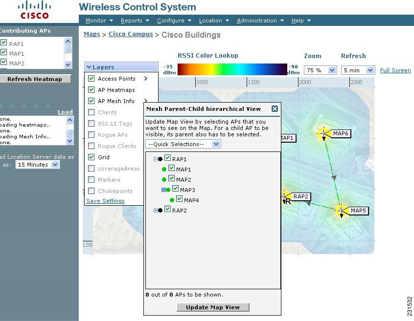
You can update the map view by choosing the access points you want to see on the map. From the Quick Selections drop-down menu, choose to select only root access point, various hops between the first and the fourth, or select all access points.
Note ![]() For a child access point to be visible, its parent must also be selected.
For a child access point to be visible, its parent must also be selected.
Clients Layer
If you enable the Clients layer and then click on the arrow to the right of these layers, a Client Filter window appears with further menu options (see Figure 5-33).
Figure 5-33 Client Filter Window
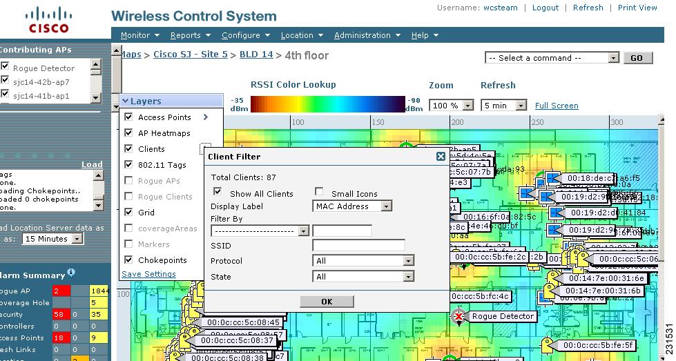
If you click the Show All Clients check box and Small Icons check box, all other drop-down menu options are grayed out.
If you uncheck the Small Icons check box, you can choose if the want the label to display MAC address, IP address, user name, asset name, asset group, or asset category.
If you uncheck the Show All Clients check box, you can specify how you want the clients filtered and enter a particular SSID.
The Protocol drop-down menu options are as follows:
•![]() All—Displays all the access points in the area.
All—Displays all the access points in the area.
•![]() 802.11a/n—Displays a colored overlay depicting the coverage patterns for the clients with 802.11a/n radios. The colors show the received signal strength from red (-35 dBm) through dark blue (-85 dBm).
802.11a/n—Displays a colored overlay depicting the coverage patterns for the clients with 802.11a/n radios. The colors show the received signal strength from red (-35 dBm) through dark blue (-85 dBm).
•![]() 802.11b/g/n—Displays a colored overlay depicting the coverage patterns for the clients with 802.11b/g/n radios. The colors show the received signal strength from red (-35 dBm) through dark blue (-85 dBm). This is the default value.
802.11b/g/n—Displays a colored overlay depicting the coverage patterns for the clients with 802.11b/g/n radios. The colors show the received signal strength from red (-35 dBm) through dark blue (-85 dBm). This is the default value.
You can further choose to show clients in all states or specifically idle, authenticated, probing, or associated clients.
802.11 Tags Layer
If you enable the 802.11 Tags layer and then click on the arrow to the right of these layers, a Tag Filter window appears with further menu options (see Figure 5-34).
Figure 5-34 Tag Filter Window
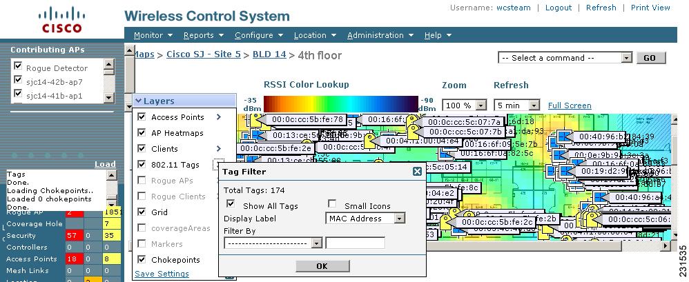
If you click the Show All Tags check box and Small Icons check box, all other drop-down menu options are grayed out.
If you uncheck the Small Icons check box, you can choose if the want the label to display MAC address, asset name, asset group, or asset category.
If you uncheck the Show All Clients check box, you can specify how you want the clients filtered.
Rogue APs Layer
If you enable the Rogue APs layer and then click on the arrow to the right of these layers, a Rogue AP Filter window appears with further menu options (see Figure 5-35).
Figure 5-35 Rogue AP Filter Window
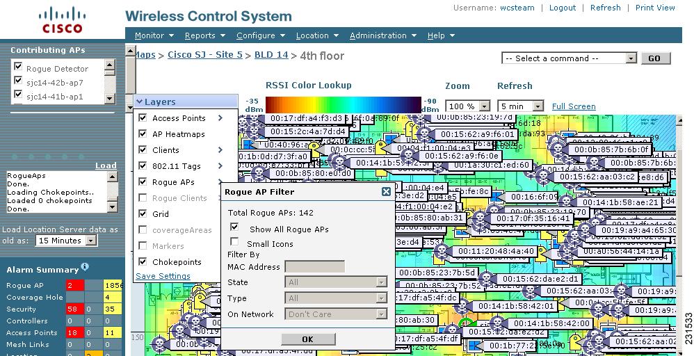
If you click the Show All Rogue APs check box and Small Icons check box, all other drop-down menu options are grayed out.
If you uncheck the Show All Rogue APs check box, you can specify how you want the rogue access points filtered. Follow these steps to define the filter.
Step 1 ![]() If you want to view a particular MAC address, enter it in the MAC Address field.
If you want to view a particular MAC address, enter it in the MAC Address field.
Step 2 ![]() From the State drop-down menu, choose if you want to display rogues in the alert, known, acknowledged, contained, threat, or unknown contained state.
From the State drop-down menu, choose if you want to display rogues in the alert, known, acknowledged, contained, threat, or unknown contained state.
Step 3 ![]() Specify if you want to display all rogues, access point rogues, or ad hoc rogues.
Specify if you want to display all rogues, access point rogues, or ad hoc rogues.
Step 4 ![]() Specify whether or not you want to display rogue access points on the network.
Specify whether or not you want to display rogue access points on the network.
Step 5 ![]() Click OK.
Click OK.
Rogue Clients Layer
If you enable the Rogue Clients layer and then click on the arrow to the right of these layers, a Rogue Client Filter window appears with further menu options (see Figure 5-36).
Figure 5-36 Rogue Client Filter Window
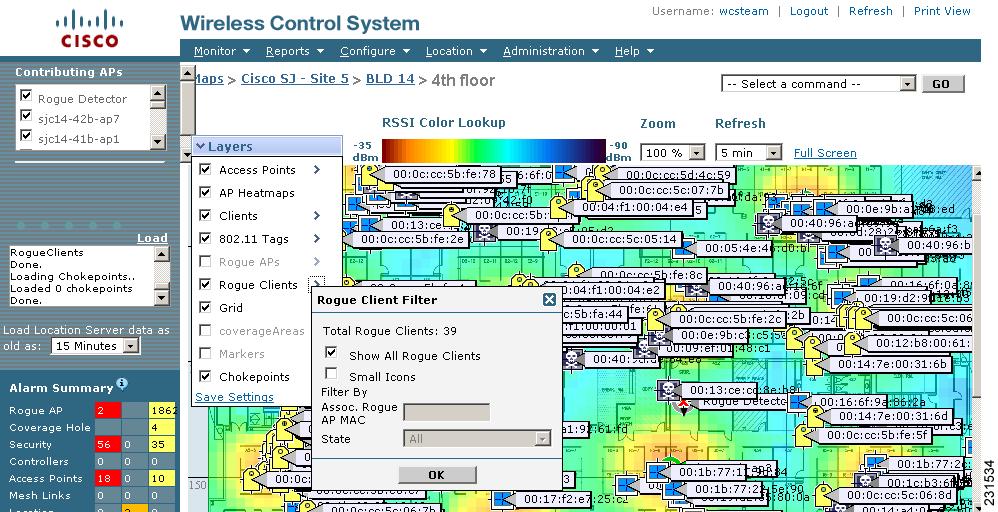
If you click the Show All Rogue Clients check box and Small Icons check box, all other drop-down menu options are grayed out.
If you uncheck the Show All Rogue Clients check box, you can specify how you want the rogue clients filtered. Follow these steps to define the filter.
Step 1 ![]() Provide the MAC address of an associated rogue access point.
Provide the MAC address of an associated rogue access point.
Step 2 ![]() Specify if you want to display all rogue clients or those in the alert, contained, or threat state.
Specify if you want to display all rogue clients or those in the alert, contained, or threat state.
Monitoring Channels on a Floor Map
Follow these steps to monitor channels on a floor map.
Step 1 ![]() Click Monitor > Maps to display the Maps page.
Click Monitor > Maps to display the Maps page.
Step 2 ![]() Click an item in the Name column.
Click an item in the Name column.
Step 3 ![]() Click >Layers.
Click >Layers.
Note ![]() When you mouse over the various locations, a popup with general, 802.11a/n, and 802.11b/g/n data appears. It provides the channel, transmit power level, user count, utilization count, antenna name, antenna angle, and elevation angle (for the 802.11a/n and 802.11b/g/n windows), and access point MAC address, model, controller IP address, location, and height in the General tab.
When you mouse over the various locations, a popup with general, 802.11a/n, and 802.11b/g/n data appears. It provides the channel, transmit power level, user count, utilization count, antenna name, antenna angle, and elevation angle (for the 802.11a/n and 802.11b/g/n windows), and access point MAC address, model, controller IP address, location, and height in the General tab.
Step 4 ![]() Click the Access Points check box.
Click the Access Points check box.
Step 5 ![]() Click the > beside Access Point.
Click the > beside Access Point.
Step 6 ![]() From the Display drop-down menu, choose Channels.
From the Display drop-down menu, choose Channels.
The number of the channel being used by each radio appears in the flag next to each access point. "Unavailable" appears for disassociated access points.
Note ![]() The available channels are defined by the country code setting and are regulated by country. Go to http://www.cisco.com/en/US/prod/collateral/wireless/ps5679/ps5861/product_data_sheet0900aecd80537b6a_ps430_Products_Data_Sheet.html.
The available channels are defined by the country code setting and are regulated by country. Go to http://www.cisco.com/en/US/prod/collateral/wireless/ps5679/ps5861/product_data_sheet0900aecd80537b6a_ps430_Products_Data_Sheet.html.
Monitoring Transmit Power Levels on a Floor Map
Follow these steps to monitor transmit power levels on a floor map.
Step 1 ![]() Click Monitor > Maps to display the Maps page.
Click Monitor > Maps to display the Maps page.
Step 2 ![]() Click an item in the Name column.
Click an item in the Name column.
Step 3 ![]() Click Layers.
Click Layers.
Note ![]() When you mouse over the various locations, a popup with general, 802.11a/n, and 802.11b/g/n data appears. It provides the channel, transmit power level, user count, utilization count, antenna name, antenna angle, and elevation angle (for the 802.11a/n and 802.11b/g/n windows), and access point MAC address, model, controller IP address, location, and height in the General tab.
When you mouse over the various locations, a popup with general, 802.11a/n, and 802.11b/g/n data appears. It provides the channel, transmit power level, user count, utilization count, antenna name, antenna angle, and elevation angle (for the 802.11a/n and 802.11b/g/n windows), and access point MAC address, model, controller IP address, location, and height in the General tab.
Step 4 ![]() Click the Access Point check box.
Click the Access Point check box.
Step 5 ![]() Click the arrow beside Access Point.
Click the arrow beside Access Point.
Step 6 ![]() Choose Tx Power Level from the Display drop-down menu.
Choose Tx Power Level from the Display drop-down menu.
Step 7 ![]() The number of the transmit power level being used by each radio appears in the flag next to each access point. "Unavailable" appears for disassociated access points.
The number of the transmit power level being used by each radio appears in the flag next to each access point. "Unavailable" appears for disassociated access points.
Table 5-4 lists the transmit power level numbers and their corresponding power settings:
|
Level Number |
|
|---|---|
1 |
Maximum power allowed per country code setting |
2 |
50% power |
3 |
25% power |
4 |
12.5 to 6.25% power |
5 |
6.25 to 0.195% power |
Note ![]() The power levels are defined by the country code setting and are regulated by country. Go to http://www.cisco.com/en/US/prod/collateral/wireless/ps5679/ps5861/product_data_sheet0900aecd80537b6a_ps430_Products_Data_Sheet.html.
The power levels are defined by the country code setting and are regulated by country. Go to http://www.cisco.com/en/US/prod/collateral/wireless/ps5679/ps5861/product_data_sheet0900aecd80537b6a_ps430_Products_Data_Sheet.html.
Monitoring Coverage Holes on a Floor Map
Coverage holes are areas in which clients cannot receive a signal from the wireless network. When you deploy a wireless network, you must consider the cost of the initial network deployment and the percentage of coverage hole areas. A reasonable coverage hole criterion for launch is between 2 and 10 percent. This means that between two and ten test locations out of 100 random test locations might receive marginal service. After launch, Cisco Unified Wireless Network Solution radio resource management (RRM) identifies these coverage hole areas and reports them to the IT manager, who can fill holes based on user demand.
Follow these steps to monitor coverage holes on a floor map.
Step 1 ![]() Click Monitor > Maps to display the Maps page.
Click Monitor > Maps to display the Maps page.
Step 2 ![]() Click an item in the Name column.
Click an item in the Name column.
Step 3 ![]() Click Layers.
Click Layers.
Note ![]() When you mouse over the various locations, a popup with general, 802.11a/n, and 802.11b/g/n data appears. It provides the channel, transmit power level, user count, utilization count, antenna name, antenna angle, and elevation angle (for the 802.11a/n and 802.11b/g/n windows), and access point MAC address, model, controller IP address, location, and height in the General tab.
When you mouse over the various locations, a popup with general, 802.11a/n, and 802.11b/g/n data appears. It provides the channel, transmit power level, user count, utilization count, antenna name, antenna angle, and elevation angle (for the 802.11a/n and 802.11b/g/n windows), and access point MAC address, model, controller IP address, location, and height in the General tab.
Step 4 ![]() Click the Access Points check box.
Click the Access Points check box.
Step 5 ![]() Click the arrow beside Access Point.
Click the arrow beside Access Point.
Step 6 ![]() Choose Coverage Holes from the Display drop-down menu.
Choose Coverage Holes from the Display drop-down menu.
The percentage of clients that have lost their connection to the wireless network appears in the flag next to each access point. "Unavailable" appears for disassociated access points, and "MonitorOnly" appears for access points in monitor-only mode.
Monitoring Clients on a Floor Map
Follow these steps to monitor client devices on a floor map.
Step 1 ![]() Click Monitor > Maps to display the Maps page.
Click Monitor > Maps to display the Maps page.
Step 2 ![]() Click an item in the Name column.
Click an item in the Name column.
Step 3 ![]() Click Layers.
Click Layers.
Note ![]() When you mouse over the various locations, a popup with general, 802.11a/n, and 802.11b/g/n data appears. It provides the channel, transmit power level, user count, utilization count, antenna name, antenna angle, and elevation angle (for the 802.11a/n and 802.11b/g/n windows), and access point MAC address, model, controller IP address, location, and height in the General tab.
When you mouse over the various locations, a popup with general, 802.11a/n, and 802.11b/g/n data appears. It provides the channel, transmit power level, user count, utilization count, antenna name, antenna angle, and elevation angle (for the 802.11a/n and 802.11b/g/n windows), and access point MAC address, model, controller IP address, location, and height in the General tab.
Step 4 ![]() Click the Access Points check box.
Click the Access Points check box.
Step 5 ![]() Click the arrow beside Access Point.
Click the arrow beside Access Point.
Step 6 ![]() Choose Users from the Display drop-down menu.
Choose Users from the Display drop-down menu.
The number of client devices associated to each radio appears in the flag next to each access point. "Unavailable" appears for disassociated access points, and "MonitorOnly" appears for access points in monitor-only mode.
Step 7 ![]() Click the number of clients to display a list of specific client devices and parameters. Table 5-5 lists the parameters that appear.
Click the number of clients to display a list of specific client devices and parameters. Table 5-5 lists the parameters that appear.
Monitoring Outdoor Areas
Follow these steps to add outdoor areas to a campus.
Step 1 ![]() Choose Monitor > Maps.
Choose Monitor > Maps.
Step 2 ![]() Click a campus name in the Name column. Verify in the Type column that it is a campus and not a building, floor area, or outdoor area.
Click a campus name in the Name column. Verify in the Type column that it is a campus and not a building, floor area, or outdoor area.
Step 3 ![]() From the Select a command drop-down menu, choose New Outdoor Area and click GO.
From the Select a command drop-down menu, choose New Outdoor Area and click GO.
Step 4 ![]() Enter the user-defined name of the new outdoor area.
Enter the user-defined name of the new outdoor area.
Step 5 ![]() Provide a contact name.
Provide a contact name.
Step 6 ![]() Use the drop-down menu to choose what type of structures exist in this area. You can choose cubes and walled offices, drywall office only, or outdoor open space.
Use the drop-down menu to choose what type of structures exist in this area. You can choose cubes and walled offices, drywall office only, or outdoor open space.
Step 7 ![]() Enter the height in feet where the access point is mounted.
Enter the height in feet where the access point is mounted.
Step 8 ![]() Enter the name of the file containing the outdoor area map or use the Browse button to locate the file. Click Next to continue with the new outdoor area process.
Enter the name of the file containing the outdoor area map or use the Browse button to locate the file. Click Next to continue with the new outdoor area process.
Step 9 ![]() A blue rectangle appears in the upper right-hand corner, superimposed on the map of the campus. Using the mouse, drag this rectangle to the desired outdoor location. To resize the blue rectangle, use Ctrl+Left+Click.
A blue rectangle appears in the upper right-hand corner, superimposed on the map of the campus. Using the mouse, drag this rectangle to the desired outdoor location. To resize the blue rectangle, use Ctrl+Left+Click.
Step 10 ![]() The name and contact information carries over to this window. Use the zoom to get a different view of the map.
The name and contact information carries over to this window. Use the zoom to get a different view of the map.
Step 11 ![]() Click the Maintain Image Aspect Ratio check box if you want to maintain the ratio of horizontal and vertical pixels of the map image. Maintaining the aspect ratio prevents visual distortion of the map.
Click the Maintain Image Aspect Ratio check box if you want to maintain the ratio of horizontal and vertical pixels of the map image. Maintaining the aspect ratio prevents visual distortion of the map.
Step 12 ![]() Enter the horizontal distance from the corner of the outdoor area rectangle to the left edge of the campus map in feet or meters.
Enter the horizontal distance from the corner of the outdoor area rectangle to the left edge of the campus map in feet or meters.
Step 13 ![]() Enter the vertical distance from the corner of the outdoor area rectangle to the top edge of the campus map in feet or meters.
Enter the vertical distance from the corner of the outdoor area rectangle to the top edge of the campus map in feet or meters.
Step 14 ![]() Enter the left to right horizontal span of the outdoor area rectangle in feet or meters.
Enter the left to right horizontal span of the outdoor area rectangle in feet or meters.
Step 15 ![]() Enter the up and down vertical span of the outdoor area rectangle in feet or meters.
Enter the up and down vertical span of the outdoor area rectangle in feet or meters.
Note ![]() To change the unit of measurement (feet or meters), choose Monitor > Maps and then choose Properties from the Select a command drop-down menu and click GO. The first drop-down menu on the Maps > Properties window allows you to choose between feet or meters as a unit of dimension.
To change the unit of measurement (feet or meters), choose Monitor > Maps and then choose Properties from the Select a command drop-down menu and click GO. The first drop-down menu on the Maps > Properties window allows you to choose between feet or meters as a unit of dimension.
Step 16 ![]() Choose Place to fix the changes on the display or Save to add them to the database.
Choose Place to fix the changes on the display or Save to add them to the database.
Importing or Exporting WLSE Map Data
When converting from autonomous to LWAPP and from WLSE to WCS, one of the conversion steps is to manually re-enter the access point-related information into WCS. This can be a time-consuming step. To speed up the process, you can export the information about access points from WLSE and import it into WCS.
Note ![]() WCS expects a .tar file and checks for a .tar extension before importing the file. If the file you are trying to import is not a .tar file, WCS displays an error message and prompts you to import a different file.
WCS expects a .tar file and checks for a .tar extension before importing the file. If the file you are trying to import is not a .tar file, WCS displays an error message and prompts you to import a different file.
To map properties and import a tar file containing WLSE data using the WCS web interface, follow these steps. For more information on the WLSE data export functionality (WLSE version 2.15), go to http://<WLSE_IP_ADDRESS>:1741/debug/export/exportSite.jsp.
Step 1 ![]() Choose Monitor > Maps.
Choose Monitor > Maps.
Step 2 ![]() Choose Properties from the Select a command drop-down menu and click GO.
Choose Properties from the Select a command drop-down menu and click GO.
Step 3 ![]() In the Import Map and AP Location section, click Browse to select the file to import.
In the Import Map and AP Location section, click Browse to select the file to import.
Step 4 ![]() Find and select the .tar file to import and click Open.
Find and select the .tar file to import and click Open.
WCS displays the name of the file in the Import From field (see Figure 5-37).
Figure 5-37 Maps > Properties Window
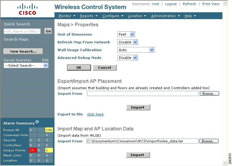
Step 5 ![]() Click Import.
Click Import.
WCS uploads the file and temporarily saves it into a local directory while it is being processed. If the file contains data that cannot be processed, WCS prompts you to correct the problem and retry. After the file has been loaded, WCS displays a report of what will be added to WCS (see Figure 5-38). The report also specifies what cannot be added and why.
Figure 5-38 Pre Execute Import Report
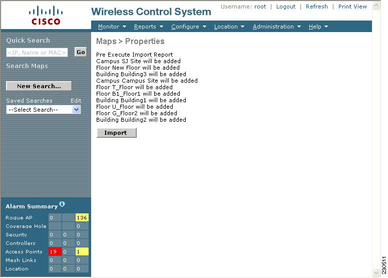
If some of the data to be imported already exists, WCS either uses the existing data in the case of campuses or overwrites the existing data using the imported data in the cases of buildings and floors (see Figure 5-39).
Figure 5-39 Pre Execute Import Report — Duplicate Data Handling
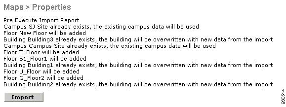
Note ![]() If there are duplicate names between a WLSE site and building combination and a WCS campus (or top-level building) and building combination, WCS displays a message in the Pre Execute Import Report indicating that it will delete the existing building.
If there are duplicate names between a WLSE site and building combination and a WCS campus (or top-level building) and building combination, WCS displays a message in the Pre Execute Import Report indicating that it will delete the existing building.
Step 6 ![]() Click Import to import the WLSE data.
Click Import to import the WLSE data.
WCS displays a report indicating what was imported (see Figure 5-40).
Figure 5-40 Post Execute Import Report
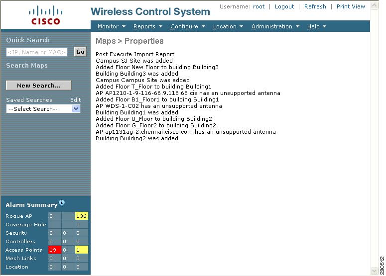
Step 7 ![]() Click Monitor > Maps to view the imported data (see Figure 5-40).
Click Monitor > Maps to view the imported data (see Figure 5-40).
Creating and Applying Calibration Models
If the provided RF models do not sufficiently characterize the floor layout, you can create a calibration model that is applied to the floor and better represents the attenuation characteristics of that floor. In environments in which many floors share common attenuation characteristics (such as in a library), one calibration model can be created and then applied to floors with the same physical layout and same deployment.
The calibration models are used as RF overlays with measured RF signal characteristics that can be applied to different floor areas. This enables the Cisco WLAN solution installation team to lay out one floor in a multi-floor area, use the RF calibration tool to measure, save the RF characteristics of that floor as a new calibration model, and apply that calibration model to all the other floors with the same physical layout.
Use a laptop or other wireless device to open a browser to the WCS server and perform the calibration process.
Step 1 ![]() Navigate to Monitor > Maps and choose RF Calibration Models from the Select a command drop-down menu. Click GO.
Navigate to Monitor > Maps and choose RF Calibration Models from the Select a command drop-down menu. Click GO.
Step 2 ![]() Choose Create New Model from the drop-down menu in the upper right. Click GO.
Choose Create New Model from the drop-down menu in the upper right. Click GO.
Step 3 ![]() Assign a name to the model and click OK.
Assign a name to the model and click OK.
Step 4 ![]() The new model appears along with the other RF calibration models, but its status is listed as Not Yet Calibrated. To start the calibration process, click on the hyperlink associated with the new model name. A new window appears which indicates the details of the new model. In the upper right-hand corner, choose Add Data Points from the drop-down menu and click GO.
The new model appears along with the other RF calibration models, but its status is listed as Not Yet Calibrated. To start the calibration process, click on the hyperlink associated with the new model name. A new window appears which indicates the details of the new model. In the upper right-hand corner, choose Add Data Points from the drop-down menu and click GO.
Step 5 ![]() If this process is being performed from a mobile device connected to WCS through the Cisco Centralized architecture, the MAC address field is automatically populated with the device's address. Otherwise, you can manually enter the MAC address of the device being used to perform the calibration. MAC addresses that are manually entered must be delimited with colons (such as FF:FF:FF:FF:FF:FF).
If this process is being performed from a mobile device connected to WCS through the Cisco Centralized architecture, the MAC address field is automatically populated with the device's address. Otherwise, you can manually enter the MAC address of the device being used to perform the calibration. MAC addresses that are manually entered must be delimited with colons (such as FF:FF:FF:FF:FF:FF).
Step 6 ![]() Choose the appropriate campus, building, and floor where the calibration is performed (see Figure 5-41). Click Next.
Choose the appropriate campus, building, and floor where the calibration is performed (see Figure 5-41). Click Next.
Figure 5-41 Starting to Calibrate
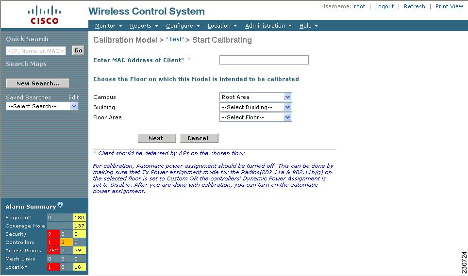
Step 7 ![]() When the chosen floor map and access point locations are presented, a grid of dots indicates the locations where data collection for calibration is performed. Using these locations as guidelines, position a wireless device in a known location on the floor. Click on the map to position the red crosshairs, indicate where the device should be located, and click Save (see Figure 5-42).
When the chosen floor map and access point locations are presented, a grid of dots indicates the locations where data collection for calibration is performed. Using these locations as guidelines, position a wireless device in a known location on the floor. Click on the map to position the red crosshairs, indicate where the device should be located, and click Save (see Figure 5-42).
Figure 5-42 Positioning the Crosshairs
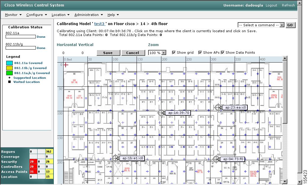
Note ![]() Use a client device that supports both 802.11a/n and 802.11b/g/n to expedite the calibration process for both spectrums.
Use a client device that supports both 802.11a/n and 802.11b/g/n to expedite the calibration process for both spectrums.
Step 8 ![]() Using the suggested location coordinates as a guideline, continue moving the mobile device throughout the floor, ensuring that the red cross hair exactly correlate with the actual location of the device. Click Save to store each location measurement.
Using the suggested location coordinates as a guideline, continue moving the mobile device throughout the floor, ensuring that the red cross hair exactly correlate with the actual location of the device. Click Save to store each location measurement.
Perform this process for each spectrum in which locationing is required until the calibration wizard shows that the process is complete. The calibration wizard shows a complete calibration after roughly 50 distinct locations and 150 measurements have been gathered. For every location point saved in the calibration process, more than one data point is gathered. Information on calibration status is provided in a legend on the left-hand side of the window. As data points are collected and areas of the map are properly calibrated, coverage is indicated by colored areas that correspond with the specific wireless LAN standard used to collect that data. The progress of the calibration process is indicated by two status bars above the legend, one for 802.11b/g/n and one for 802.11a/n.
Step 9 ![]() When the calibration is complete for each spectrum in which locationing is required, click on the name of the calibration model at the top of the window to return to the main screen for that model.
When the calibration is complete for each spectrum in which locationing is required, click on the name of the calibration model at the top of the window to return to the main screen for that model.
Step 10 ![]() After all the raw data collection is performed, compile the model, and then WCS and the location appliance use the data to understand RF attenuation characteristics. To compute the collected data points, choose Calibrate from the drop-down menu and click GO.
After all the raw data collection is performed, compile the model, and then WCS and the location appliance use the data to understand RF attenuation characteristics. To compute the collected data points, choose Calibrate from the drop-down menu and click GO.
Step 11 ![]() To use the newly created calibration model, you must apply the model to the floor on which it was created (and on any other floors with similar attenuation characteristics as well). Navigate to Monitor > Maps and find the specific floor to which the model is applied. At the floor map interface, choose Edit Floor Area from the drop-down menu and click GO.
To use the newly created calibration model, you must apply the model to the floor on which it was created (and on any other floors with similar attenuation characteristics as well). Navigate to Monitor > Maps and find the specific floor to which the model is applied. At the floor map interface, choose Edit Floor Area from the drop-down menu and click GO.
Step 12 ![]() From the Floor Type (RF Model) drop-down menu, choose the newly created calibration model. Click OK to apply the model to the floor.
From the Floor Type (RF Model) drop-down menu, choose the newly created calibration model. Click OK to apply the model to the floor.
Note ![]() This process can be repeated for as many models and floors as needed. After a model is applied to a floor, all location determination performed on that floor is done using the specific collected attenuation data from the calibration model.
This process can be repeated for as many models and floors as needed. After a model is applied to a floor, all location determination performed on that floor is done using the specific collected attenuation data from the calibration model.
Analyzing Element Location Accuracy Using Testpoints
You can analyze the location accuracy of rogue and non-rogue clients and asset tags by entering testpoints on an area or floor map. You can use this feature to validate location information generated either automatically by access points or manually by calibration.
Note ![]() By checking for location accuracy, you are checking the ability of the existing access point deployment to estimate the true location of an element within 10 meters at least 90% of the time.
By checking for location accuracy, you are checking the ability of the existing access point deployment to estimate the true location of an element within 10 meters at least 90% of the time.
Note ![]() Before starting this process, record the MAC addresses and locations for all elements within the area or floor to be analyzed. You need this information when placing the testpoints on the map. If analyzing location after calibration, you should analyze the location accuracy of at least as many elements entered during calibration.
Before starting this process, record the MAC addresses and locations for all elements within the area or floor to be analyzed. You need this information when placing the testpoints on the map. If analyzing location after calibration, you should analyze the location accuracy of at least as many elements entered during calibration.
Note ![]() The Advanced Debug option must be enabled on both the location appliance and WCS to allow use of the location accuracy testpoint feature.
The Advanced Debug option must be enabled on both the location appliance and WCS to allow use of the location accuracy testpoint feature.
Follow these steps to enable the advanced debug option and assign testpoints to a floor map to check location accuracy.
Step 1 ![]() Choose Location > Location Servers.
Choose Location > Location Servers.
Step 2 ![]() Select a server from the All Location Servers page that appears.
Select a server from the All Location Servers page that appears.
Step 3 ![]() Select Advanced Parameters from the Administration menu of the Location Server General Properties page (see Figure 5-43).
Select Advanced Parameters from the Administration menu of the Location Server General Properties page (see Figure 5-43).
Figure 5-43 Location Server General Properties Page
Step 4 ![]() On the page that appears, scroll down to the Advanced Parameters section. Check the Advanced Debug box to enable the feature. Click Save.
On the page that appears, scroll down to the Advanced Parameters section. Check the Advanced Debug box to enable the feature. Click Save.
Note ![]() If the Advanced Debug check box is already checked, you do not need to do anything further. Click Cancel.
If the Advanced Debug check box is already checked, you do not need to do anything further. Click Cancel.
Assigning Testpoints to a Selected Area
You now must enable the Advanced debug level at the Maps level and begin assigning testpoints to a selected area or map.
Step 1 ![]() Choose Monitor > Maps.
Choose Monitor > Maps.
Step 2 ![]() Select Properties from the Select a command drop-down menu.
Select Properties from the Select a command drop-down menu.
Step 3 ![]() On the Maps > Properties page (see Figure 5-44), select Enable from the Advanced Debug drop-down menu. Click OK.
On the Maps > Properties page (see Figure 5-44), select Enable from the Advanced Debug drop-down menu. Click OK.
Figure 5-44 Map > Properties Page
You are returned to the Maps summary window. You are now ready to assign testpoints to a selected area or map.
Step 4 ![]() Choose Monitor > Maps. Select the area or floor you want to analyze from the map summary that appears.
Choose Monitor > Maps. Select the area or floor you want to analyze from the map summary that appears.
The page seen in Figure 5-45 appears.
Figure 5-45 Selected Area or Floor Map Chosen at Monitor > Maps Page
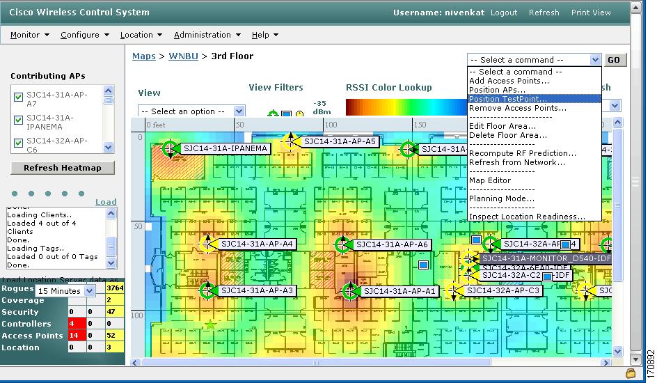
Step 5 ![]() Select Position TestPoint from the Select a command drop-down menu (top-right). Click GO.
Select Position TestPoint from the Select a command drop-down menu (top-right). Click GO.
A blank map of the selected area or floor appears for testpoint assignment (see Figure 5-46).
Figure 5-46 Position TestPoint Assignment Page
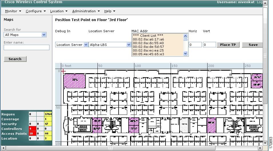
Step 6 ![]() On the Position Test Point page, select the location server from the drop-down menu and choose a MAC address from the list of MAC addresses (for clients, tags, rogue access point, rogue clients, and so on).
On the Position Test Point page, select the location server from the drop-down menu and choose a MAC address from the list of MAC addresses (for clients, tags, rogue access point, rogue clients, and so on).
Note ![]() If you entered horizontal and vertical coordinates, click Place TP instead of Save.
If you entered horizontal and vertical coordinates, click Place TP instead of Save.
Step 7 ![]() Move the red cross-hair cursor (top-left) to the map location that corresponds to the actual position of the element and click Save.
Move the red cross-hair cursor (top-left) to the map location that corresponds to the actual position of the element and click Save.
Note ![]() Instead of using the cursor, you can enter the horizontal (Horz) and vertical (Vert) coordinates of the asset tag or client to mark its location.
Instead of using the cursor, you can enter the horizontal (Horz) and vertical (Vert) coordinates of the asset tag or client to mark its location.
A pop up box appears noting successful addition of the testpoint for the element and its MAC address.
The red cross hair cursor returns to the upper left-band corner after placement is confirmed. You are ready to mark additional testpoints.
Step 8 ![]() Wait 2 minutes to collect enough data to analyze. After waiting at least 2 minutes, click Stop.
Wait 2 minutes to collect enough data to analyze. After waiting at least 2 minutes, click Stop.
Note ![]() If you wait less than 2 minutes before clicking Stop, the accuracy of the data is deteriorated.
If you wait less than 2 minutes before clicking Stop, the accuracy of the data is deteriorated.
Step 9 ![]() Repeat Steps 6 and 7 for each client or asset tag you want to add to the map.
Repeat Steps 6 and 7 for each client or asset tag you want to add to the map.
Step 10 ![]() Click Analyze (far-right) to determine location accuracy of the entered testpoints.
Click Analyze (far-right) to determine location accuracy of the entered testpoints.
A pop up window appears providing accuracy percentage and the number of sample points gathered during that interval.
You can perform this test for multiple elements by selecting multiple MAC addresses from the list of MAC addresses and repeating the above procedure.
 Feedback