Cisco UCS Integrated Infrastructure for Big Data and Analytics with Cloudera and Apache Spark
Available Languages

Cisco UCS Integrated Infrastructure for Big Data and Analytics with Cloudera and Apache Spark
Building a 64 Node Hadoop Cluster
Last Updated: June 29, 2016

The CVD program consists of systems and solutions designed, tested, and documented to facilitate faster, more reliable, and more predictable customer deployments. For more information visit
http://www.cisco.com/go/designzone.
ALL DESIGNS, SPECIFICATIONS, STATEMENTS, INFORMATION, AND RECOMMENDATIONS (COLLECTIVELY, "DESIGNS") IN THIS MANUAL ARE PRESENTED "AS IS," WITH ALL FAULTS. CISCO AND ITS SUPPLIERS DISCLAIM ALL WARRANTIES, INCLUDING, WITHOUT LIMITATION, THE WARRANTY OF MERCHANTABILITY, FITNESS FOR A PARTICULAR PURPOSE AND NONINFRINGEMENT OR ARISING FROM A COURSE OF DEALING, USAGE, OR TRADE PRACTICE. IN NO EVENT SHALL CISCO OR ITS SUPPLIERS BE LIABLE FOR ANY INDIRECT, SPECIAL, CONSEQUENTIAL, OR INCIDENTAL DAMAGES, INCLUDING, WITHOUT LIMITATION, LOST PROFITS OR LOSS OR DAMAGE TO DATA ARISING OUT OF THE USE OR INABILITY TO USE THE DESIGNS, EVEN IF CISCO OR ITS SUPPLIERS HAVE BEEN ADVISED OF THE POSSIBILITY OF SUCH DAMAGES.
THE DESIGNS ARE SUBJECT TO CHANGE WITHOUT NOTICE. USERS ARE SOLELY RESPONSIBLE FOR THEIR APPLICATION OF THE DESIGNS. THE DESIGNS DO NOT CONSTITUTE THE TECHNICAL OR OTHER PROFESSIONAL ADVICE OF CISCO, ITS SUPPLIERS OR PARTNERS. USERS SHOULD CONSULT THEIR OWN TECHNICAL ADVISORS BEFORE IMPLEMENTING THE DESIGNS. RESULTS MAY VARY DEPENDING ON FACTORS NOT TESTED BY CISCO.
CCDE, CCENT, Cisco Eos, Cisco Lumin, Cisco Nexus, Cisco StadiumVision, Cisco TelePresence, Cisco WebEx, the Cisco logo, DCE, and Welcome to the Human Network are trademarks; Changing the Way We Work, Live, Play, and Learn and Cisco Store are service marks; and Access Registrar, Aironet, AsyncOS, Bringing the Meeting To You, Catalyst, CCDA, CCDP, CCIE, CCIP, CCNA, CCNP, CCSP, CCVP, Cisco, the Cisco Certified Internetwork Expert logo, Cisco IOS, Cisco Press, Cisco Systems, Cisco Systems Capital, the Cisco Systems logo, Cisco Unity, Collaboration Without Limitation, EtherFast, EtherSwitch, Event Center, Fast Step, Follow Me Browsing, FormShare, GigaDrive, HomeLink, Internet Quotient, IOS, iPhone, iQuick Study, IronPort, the IronPort logo, LightStream, Linksys, MediaTone, MeetingPlace, MeetingPlace Chime Sound, MGX, Networkers, Networking Academy, Network Registrar, PCNow, PIX, PowerPanels, ProConnect, ScriptShare, SenderBase, SMARTnet, Spectrum Expert, StackWise, The Fastest Way to Increase Your Internet Quotient, TransPath, WebEx, and the WebEx logo are registered trademarks of Cisco Systems, Inc. and/or its affiliates in the United States and certain other countries.
All other trademarks mentioned in this document or website are the property of their respective owners. The use of the word partner does not imply a partnership relationship between Cisco and any other company. (0809R)
© 2016 Cisco Systems, Inc. All rights reserved.
Table of Contents
Big Data Processing with Apache Spark
Scaling and Sizing the Cluster for Spark Streaming with Kafka
Cisco UCS Integrated Infrastructure for Big Data and Analytics with Cloudera
Cisco UCS 6200 Series Fabric Interconnects
Cisco UCS 6300 Series Fabric Interconnects
Cisco UCS C-Series Rack Mount Servers
Cisco UCS Virtual Interface Cards (VICs)
Port Configuration on Fabric Interconnects
Server Configuration and Cabling for C240M4
Software Distributions and Versions
Red Hat Enterprise Linux (RHEL)
Performing Initial Setup of Cisco UCS 6296 Fabric Interconnects
Configure Fabric Interconnect A
Configure Fabric Interconnect B
Logging Into Cisco UCS Manager
Upgrading UCSM Software to Version 3.1(1g)
Adding a Block of IP Addresses for KVM Access
Creating Pools for Service Profile Templates
Creating Policies for Service Profile Templates
Creating Host Firmware Package Policy
Creating the Local Disk Configuration Policy
Creating a Service Profile Template
Configuring the Storage Provisioning for the Template
Configuring Network Settings for the Template
Configuring the vMedia Policy for the Template
Configuring Server Boot Order for the Template
Configuring Server Assignment for the Template
Configuring Operational Policies for the Template
Installing Red Hat Enterprise Linux 7.2
Setting Up Password-less Login
Creating a Red Hat Enterprise Linux (RHEL) 7.2 Local Repo
Creating the Red Hat Repository Database.
Set Up all Nodes to use the RHEL Repository
Upgrading the Cisco Network driver for VIC1227
Disable Transparent Huge Pages
Configuring Data Drives on Name Node And Other Management Nodes
Configuring Data Drives on Data Nodes
Configuring the Filesystem for NameNodes and Datanodes
Pre-Requisites for CDH Installation
Setting up the Local Parcels for CDH 5.7.0
Setting Up the MariaDB Database for Cloudera Manager
Setting Up the Cloudera Manager Server Database
Starting The Cloudera Manager Server
Installing Cloudera Enterprise Data Hub (CDH5)
Configuring Hue to Work with HDFS HA
Configuring Yarn (MR2 Included) and HDFS Services
Apache Kafka Installation and Configuration
Tuning Resource Allocation for Spark
Shuffle performance improvement
Improving Serialization performance
Changing the Log Directory for All Applications
Big Data technology is commonly categorized into management, storage, and processing of a huge volume, velocity, and variety of data. Hadoop, which is the most popular Big Data technology, is designed to handle these massive amounts of data very well. Big Data has always been synonymous with high-throughput Batch Processing systems that can crunch huge volumes of data using distributed parallel processing for excellent offline data processing. Real-Time/Near Real-Time processing is the natural progression from Batch Processing. Real-Time Systems also need to process the data but additionally they need to guarantee the response within specific time constraints, and return results that will affect the environment they are running in. Numerous use cases are emerging across various verticals that need super fast responses from Big Data for faster decision-making.
A powerful, easy-to-use open source platform for these use cases is Apache Spark. With its in-memory capabilities, it offers both real-time and batch processing capabilities over a wide range of scenarios. Some of the use cases Spark is well suited for include credit card fraud analytics, network fault prediction, security threats, IoT sensor analytics, machine data analytics, integrated complex analytics with interactive applications, sentiment analytics on social media data, etc. With Apache Spark, both analytic workloads and real-time events can be passed to clustering algorithms and this could be federated with other data sources to find insights in real-time.
Cisco UCS Integrated Infrastructure for Big Data and Analytics with Cloudera Enterprise is a dependable deployment model for Hadoop with Spark while offering a fast and predictable path for businesses to unlock value in Big Data. The configuration detailed in the document can be scaled to clusters of various sizes depending on the application demand. Up to 80 servers (5 racks) can be supported with no additional switching in a single UCS domain. Scaling beyond 5 racks (80 servers) can be implemented by interconnecting multiple UCS domains using Nexus 9000 Series switches or Cisco Application Centric Infrastructure (ACI), scalable to thousands of servers and to hundreds of petabytes of storage, and managed from a single pane using Cisco UCS Central.
Introduction
Hadoop is a strategic data platform embraced by mainstream enterprises. Now combined with Apache Spark, a fast in-memory cluster-computing framework, it offers the fastest path for businesses to unlock value in Big Data while maximizing existing investments.
Real time data processing involves a continual input, process and output of data. Data must be processed in a small time period (or near real time). Real time data processing and analytics allows an organization the ability to take immediate action for those times when acting within seconds or minutes is significant. The goal is to obtain the insight required to act prudently at the right time - which increasingly means immediately.
Industries are trying to capitalize on these new business insights to drive competitive advantage. Apache Hadoop is the most common Big Data framework, and the technology is evolving rapidly – and one of the latest innovations is Apache Spark.
Solution
This solution brings a simple and linearly scalable architecture to provide Apache Spark on the Cloudera Platform with Apache Hadoop (CDH), that can cater to both batch and real time processing with a centrally managed automated Hadoop deployment, providing all the benefits of the Cisco UCS Integrated Infrastructure for Big Data and Analytics.
With this solution you can deploy Spark on any existing Hadoop cluster, or on a completely new cluster. This installation will cater to Batch processing, but also to Stream processing, combined with other technologies like Flume, and Kafka, etc.
Some of the features of this solution include:
· Infrastructure for both Big Data and Streaming Analytics.
· Simplified infrastructure management via Cisco UCS Manager.
· Flexible Big Data platform, which works for both batch and real time processing.
· Architectural Scalability, linear scaling based on data requirements.
· Usage of Cloudera Enterprise for comprehensive cluster monitoring and management.
This solution is based on the Cisco UCS Integrated Infrastructure for Big Data and Analytics and includes computing, storage, connectivity, and unified management capabilities to help companies manage the immense amount of data they collect today. It is built on the Cisco Unified Computing System (Cisco UCS) infrastructure, using Cisco UCS 6200 Series Fabric Interconnects, and Cisco UCS C-Series Rack Servers. This architecture is specifically designed for performance and linear scalability for Big Data workloads.
Audience
This document describes the architecture and deployment procedures for Cloudera on a 64 Cisco UCS C240 M4 node cluster based on Cisco UCS Integrated Infrastructure for Big Data and Analytics. The intended audience for this document includes, but is not limited to, sales engineers, field consultants, professional services, IT managers, partner engineering, and customers who want to deploy Cloudera Distribution with Apache Hadoop (CDH 5.7) on Cisco UCS Integrated Infrastructure for Big Data and Analytics.
Solution Summary
This CVD describes in detail the process of installing Cloudera 5.7.0 with Apache Spark and the configuration details of the cluster. It also details application configuration for Spark and the libraries it provides, and the best practices and guidelines for running Spark Applications. It also has details on adding in Kafka clusters managed using Cloudera and relevant configurations. The current version of Cisco UCS Integrated Infrastructure for Big Data and Analytics offers the following configurations depending on the compute and storage requirements as shown in Table 1 .
Table 1 Cisco UCS Integrated Infrastructure for Big Data and Analytics Configuration Details
| Performance Optimized Option 1 (UCS-SL-CPA4 -P1) |
Performance Optimized Option 2 (UCS-SL-CPA4 -P2) |
Performance Optimized Option 3 UCS-SL-CPA4-P3 |
Capacity Optimized Option 1 UCS-SL-CPA4-C1 |
Capacity Optimized Option 2 UCS-SL-CPA4-C2 |
| 2 Cisco UCS 6296 UP, 96 port Fabric Interconnects |
2 Cisco UCS 6296 UP, 96 port Fabric Interconnects |
2 Cisco UCS 6332 Fabric Interconnects |
2 Cisco UCS 6296 UP, 96 port Fabric Interconnects |
2 Cisco UCS 6296 UP, 96 port Fabric Interconnects |
| 16 Cisco UCS C240 M4 Rack Servers (SFF), each with: |
16 Cisco UCS C240 M4 Rack Servers (SFF), each with: |
16 Cisco UCS C240 M4 Rack Servers (SFF), each with: |
16 Cisco UCS C240 M4 Rack Servers (LFF), each with: |
16 Cisco UCS C240 M4 Rack Servers (LFF), each with: |
| 2 Intel Xeon processors E5-2680 v4 CPUs (14 cores on each CPU) |
2 Intel Xeon processors E5-2680 v4 CPUs (14 cores on each CPU) |
2 Intel Xeon processors E5-2680 v4 CPUs (14 cores on each CPU) |
2 Intel Xeon processors E5-2620 v4 CPUs (8 cores each CPU) |
2 Intel Xeon processors E5-2620 v4 CPUs (8 cores each CPU) |
| 256 GB of memory |
256 GB of memory |
256 GB of memory |
128 GB of memory |
256 GB of memory |
| Cisco 12-Gbps SAS Modular Raid Controller with 2-GB flash-based write cache (FBWC) |
Cisco 12-Gbps SAS Modular Raid Controller with 2-GB flash-based write cache (FBWC) |
Cisco 12-Gbps SAS Modular Raid Controller with 2-GB flash-based write cache (FBWC) |
Cisco 12-Gbps SAS Modular Raid Controller with 2-GB flash-based write cache (FBWC) |
Cisco 12-Gbps SAS Modular Raid Controller with 2-GB flash-based write cache (FBWC) |
| 24 1.2-TB 10K SFF SAS drives (460 TB total) |
24 1.8-TB 10K SFF SAS drives (691 TB total) |
24 1.8-TB 10K SFF SAS drives (691 TB total) |
12 6-TB 7.2K LFF SAS drives (1152 TB total) |
12 8-TB 7.2K LFF SAS drives (1536 TB total) |
| 2 240-GB 6-Gbps 2.5-inch Enterprise Value SATA SSDs for Boot |
2 240-GB 6-Gbps 2.5-inch Enterprise Value SATA SSDs for Boot |
2 240-GB 6-Gbps 2.5-inch Enterprise Value SATA SSDs for Boot |
2 240-GB 6-Gbps 2.5-inch Enterprise Value SATA SSDs for Boot |
2 240-GB 6-Gbps 2.5-inch Enterprise Value SATA SSDs for Boot |
| Cisco UCS VIC 1227 (with 2 10 GE SFP+ ports) |
Cisco UCS VIC 1227 (with 2 10 GE SFP+ ports) |
Cisco UCS VIC 1387 (with 2 40 GE SFP+ ports) |
Cisco UCS VIC 1227 (with 2 10 GE SFP+ ports) |
Cisco UCS VIC 1227 (with 2 10 GE SFP+ ports) |
Big Data Processing with Apache Spark
As companies realize the power of Big Data, they are collecting more data than ever and realize the need to get value from data in real-time. Sensors, IoT devices, Social Network data and online transactions, etc., are all generating data that has to be captured, monitored, and processed quickly, in some cases to make fast, data-derived decisions. Also this data being collected in stream is most likely to be processed and used in batch jobs for generating daily reports or updating the parameters to the existing machine-learning models.
Spark is a data processing framework with a unified programming model that provides support for a variety of workloads like batch, and streaming, and can perform both interactive and iterative processing through a powerful set of built-in libraries – Spark Core, Spark Streaming, Spark SQL, MLlib, GraphX. The internal details of these libraries are described below in the Technology Overview section of this document.
Spark enables applications in Hadoop clusters to run faster as it allows caching datasets, so the data can now be available on RAM instead of disk. That improves the performance of especially iterative algorithms that access the same dataset repeatedly. In addition to Map and Reduce operations, additional operations like SQL queries, Machine learning and Graph Data processing can be performed. Spark allows programmers to develop complex, multi-step data pipelines using directed acyclic graph (DAG) patterns. It also supports in-memory data sharing across DAGs, so that different jobs can work with the same data.
Spark Streaming Processing
Both Edge and Stream Analytics with Spark, in combination with Apache Kafka or Fog Nodes, are becoming very common in the industry. Dashboards and visualization software on top of these analytics platforms are helping enterprises to visualize and monitor their business in real-time.
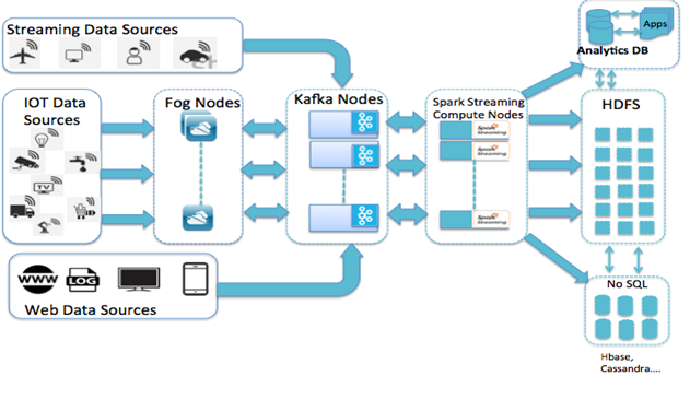
The figure below depicts the data flow for Spark Stream Processing that covers most typical use cases for Spark. Data is collected from various sources IoT sensors, streaming sources that are sending data daily, hourly, per minute, and data from online sources, etc. This data is accumulated using Fog Nodes in combination with Apache Kafka, (a publish-subscribe distributed messaging system), or Apache Flume, (a distributed HA service for efficiently collecting, aggregating and moving large amounts of streaming event data), and then processed using Spark Streaming.
Apache Flume is easily integrated into an existing Hadoop infrastructure, Apache Kafka as a channel, and HDFS as a sink. A Flume agent will read events from Kafka and write them to HDFS, HBase or Solr, from which they can be accessed by Spark, Impala, Hive, or other BI tools.
The working details of implementing Apache Flume, and the architecture of Flume is described in the Technology Overview section of this document.
Kafka’s popularity can be attributed to its design and operational simplicity. Kafka has stronger ordering guarantees than traditional messaging systems, and the data replication can be easily tuned for varying sized workloads. Spark streaming jobs output is only as reliable as the queue that feeds into Spark, so using a technology like Kafka is very popular.
Spark allows engineers to test an application in batch mode and move it to streaming mode easily. Spark Streaming mode enables organizations to get insights from data in the last one minute, or last hour. This data can be consumed into SQL, or NO SQL databases that power real-time dashboards, or are used in machine-learning models, or in Elastic, Solr, etc., to build indices for powering Enterprise searches or Analytics.
Figure 1 below is a flowchart that captures most of these use cases and how the data-flow moves from various Data Sources into Fog Nodes or Kafka, and then into Spark, and further downstream into HDFS, HBase, etc.
Figure 1 Typical Data Flow for Stream Processing
With the ability to react and make prompt decisions based on real-time processing, more businesses are beginning to expand beyond batch-processing methods, to build new data products using Spark Streaming. Building applications on these platforms that can scale, reliably process data without any loss, satisfy the business and functional requirements, and honor the latency requirements, requires the system to be designed well, and the software to be tuned well. Understanding these requirements, and after working with various business verticals, the next section details the relevant reference architectures utilizing the power of Spark on the Cisco UCS Integrated Infrastructure for Big Data and Analytics.
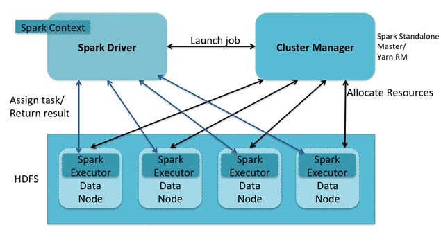
Figure 2 below shows a detailed flow chart of how a Spark application executes on a HDFS cluster.
Figure 2 Spark Application Architecture
Spark Reference Architecture
Figure 3 shows the base configuration of 64 nodes with SFF (1.8TB) drives. This also offers HA of the cluster with 3 management nodes.
Figure 3 Reference Architecture for Spark

![]() Note: This CVD describes the installation process of CDH 5.7.0 for a 64 node (3 Management Nodes for HA + 61 Data Nodes) on a Performance Optimized Option 2 Cluster configuration. It also has details on how to add in Kafka if needed as part of the same cluster.
Note: This CVD describes the installation process of CDH 5.7.0 for a 64 node (3 Management Nodes for HA + 61 Data Nodes) on a Performance Optimized Option 2 Cluster configuration. It also has details on how to add in Kafka if needed as part of the same cluster.
![]() Note: If a customer decides to use the 6300 series FI (40 G connectivity) for the configuration, instead of the 6200 series FI in Performance Optimized Option 2, the only change will be to add in the Cisco VIC 1387, the rest of the configuration will be exactly the same.
Note: If a customer decides to use the 6300 series FI (40 G connectivity) for the configuration, instead of the 6200 series FI in Performance Optimized Option 2, the only change will be to add in the Cisco VIC 1387, the rest of the configuration will be exactly the same.
Figure 4 shows the reference architecture for the complete streaming architecture with Kafka included for streaming data into the Hadoop cluster.
Figure 4 Reference Architecture for Spark Streaming with Kafka
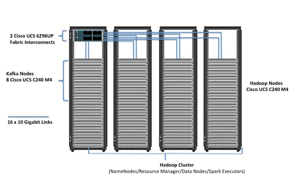
![]() Note: In Figure 4 above, Kafka is managed as part of the Hadoop cluster, and deployed and managed using Cloudera Manager.
Note: In Figure 4 above, Kafka is managed as part of the Hadoop cluster, and deployed and managed using Cloudera Manager.
Table 2 Configuration Details
| Component |
Description |
| Connectivity |
2 Cisco UCS 6296UP 96-Port Fabric Interconnects Up to 80 servers with no additional switching infrastructure |
| Hadoop Cluster |
64 Cisco UCS C240 M4 Rack Servers Hadoop NameNode/Secondary NameNode and Resource Manager and Data Nodes. Spark Executors are collocated on a Data Node. *Please refer to Service Assignment section for specific service assignment and configuration details. |
| Kafka Nodes |
8 Cisco UCS C240 M4 Rack Servers Same as Data Nodes |
Scaling and Sizing the Cluster for Spark Streaming with Kafka
To scale the Streaming Architecture while utilizing Kafka, Table 3 shows the scaling and sizing guidelines for Kafka storage, for various drives, and replication factors.
Time taken for filling one server = ~((Total Storage)/Network Bandwidth)/3600)
Table 3 Scaling and Sizing Guidelines
| Network Bandwidth |
Server Type |
Total Usable Storage |
Time Taken to Fill One server |
Total Servers |
Total Servers |
|
|
|
|
|
(1 way replicated data) (Full network utilization) |
(3 way replicated data) (Full network utilization) |
| 10 Gbps (1.25 GBps) |
C240 M4 (SFF) with 1.8 TB drives |
~40800 GB |
~9 hours |
~3 servers for storing 1 day of data |
~9 servers for storing 1 day of data |
| 40 Gbps (5 GBps) |
C240 M4 (SFF) with 1.8 TB drives |
~40800 GB |
~2.3 hours |
~10 servers for storing 1 day of data |
~30 servers for storing 1 day of data ( |
| 10 Gbps (1.25 GBps) |
C240 M4 (LFF) with 6 TB drives |
~72000 GB |
~16 hours |
~2 servers for storing 1 day of data |
~6 servers for storing 1 day of data |
| 40 Gbps |
C240 M4 (LFF) with 6 TB drives |
~72000 GB |
~4 hours |
~ 6 servers for storing 1 day of data |
~18 servers for storing 1 day of data |
Cisco UCS Integrated Infrastructure for Big Data and Analytics with Cloudera
The Cisco UCS Integrated Infrastructure for Big Data and Analytics solution for Cloudera is based on Cisco UCS Integrated Infrastructure for Big Data and Analytics, a highly scalable architecture designed to meet a variety of scale-out application demands with seamless data integration, and management integration capabilities, built using the following components:
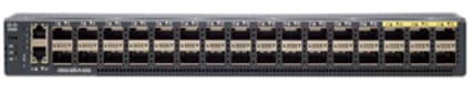
Cisco UCS 6200 Series Fabric Interconnects
Cisco UCS 6200 Series Fabric Interconnects provide high-bandwidth, low-latency connectivity for servers, with integrated, unified management provided for all connected devices by Cisco UCS Manager. Deployed in redundant pairs, Cisco fabric interconnects offer the full active-active redundancy, performance, and exceptional scalability needed to support the large number of nodes that are typical in clusters serving Big Data applications. Cisco UCS Manager enables rapid and consistent server configuration using service profiles, automating ongoing system maintenance activities such as firmware updates across the entire cluster as a single operation. Cisco UCS Manager also offers advanced monitoring, with options to raise alarms, and send notifications about the health of the entire cluster.
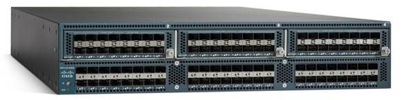
Figure 5 Cisco UCS 6296UP 96-Port Fabric Interconnect
Cisco UCS 6300 Series Fabric Interconnects
Cisco UCS 6300 Series Fabric Interconnects is the new series of Fabric Interconnects that Cisco has introduced. The Cisco UCS 6300 series Fabric interconnects are a core part of Cisco UCS, providing low-latency, lossless 10 and 40 Gigabit Ethernet, Fiber Channel over Ethernet (FCoE), and Fiber Channel functions with management capabilities for the system. All servers attached to Fabric interconnects become part of a single, highly-available management domain.
Figure 6 Cisco UCS 6332 UP 32 -Port Fabric Interconnect
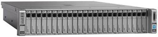
Cisco UCS C-Series Rack Mount Servers
Cisco UCS C-Series Rack Mount C220 M4 High-Density Rack Servers (Small Form Factor Disk Drive Model), and Cisco UCS C240 M4 High-Density Rack Servers (Small Form Factor Disk Drive Model), are enterprise-class systems that support a wide range of computing, I/O, and storage-capacity demands in compact designs. Cisco UCS C-Series Rack-Mount Servers are based on the Intel Xeon E5-2600 v3 and v4 series processor family that delivers the best combination of performance, flexibility, and efficiency gains, with 12-Gbps SAS throughput. The Cisco UCS C240 M4 servers provide 24 DIMM (PCIe) 3.0 slots and can support up to 768 GB of main memory, (128 or 256 GB is typical for Big Data applications). It can support a range of disk drive and SSD options; twenty-four Small Form Factor (SFF) disk drives plus two (optional) internal SATA boot drives, for a total of 26 internal drives, are supported in the Performance Optimized option. Twelve Large Form Factor (LFF) disk drives, plus two (optional) internal SATA boot drives, for a total of 14 internal drives, are supported in the Capacity Optimized option, along with 2x1 Gigabit Ethernet embedded LAN-on-motherboard (LOM) ports. Cisco UCS Virtual Interface Cards 1227 (VICs), designed for the M4 generation of Cisco UCS C-Series Rack Servers, are optimized for high-bandwidth and low-latency cluster connectivity, with support for up to 256 virtual devices, that are configured on demand through Cisco UCS Manager.
Figure 7 Cisco UCS C240 M4 Rack Server
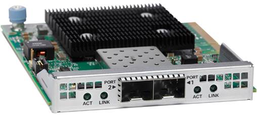
Cisco UCS Virtual Interface Cards (VICs)
Cisco UCS Virtual Interface Cards (VICs) are unique to Cisco. Cisco UCS Virtual Interface Cards incorporate next-generation converged network adapter (CNA) technology from Cisco, and offer dual 10-Gbps ports designed for use with Cisco UCS C-Series Rack-Mount Servers. Optimized for virtualized networking, these cards deliver high performance and bandwidth utilization, and support up to 256 virtual devices. The Cisco UCS Virtual Interface Card (VIC) 1227 is a dual-port, Enhanced Small Form-Factor Pluggable (SFP+), 10 Gigabit Ethernet, and Fiber Channel over Ethernet (FCoE)-capable, PCI Express (PCIe) modular LAN on motherboard (mLOM) adapter.
Figure 8 Cisco UCS VIC 1227
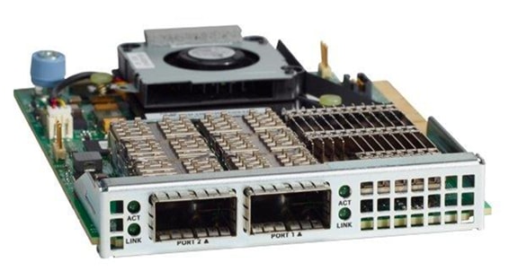
The Cisco UCS Virtual Interface Card 1387 offers dual-port, Enhanced Quad, Small Form-Factor Pluggable (QSFP+) 40 Gigabit Ethernet and Fiber Channel over Ethernet (FCoE), in a modular-LAN-on-motherboard (mLOM) form factor. The mLOM slot can be used to install a Cisco VIC without consuming a PCIe slot providing greater I/O expandability.
Figure 9 Cisco UCS VIC 1387
Cisco UCS Manager
Cisco UCS Manager resides within the Cisco UCS 6200 Series Fabric Interconnect. It makes the system self-aware and self-integrating, managing all of the system components as a single logical entity. Cisco UCS Manager can be accessed through an intuitive graphical user interface (GUI), a command-line interface (CLI), or an XML application-programming interface (API). Cisco UCS Manager uses service profiles to define the personality, configuration, and connectivity of all resources within Cisco UCS, radically simplifying provisioning of resources so the process takes minutes instead of days. This simplification allows IT departments to shift their focus from constant maintenance to strategic business initiatives.
Figure 10 Cisco UCS Manager
Cloudera (CDH 5.7.0)
Built on the transformative Apache Hadoop open source software project, Cloudera Enterprise is a hardened distribution of Apache Hadoop and related projects designed for the demanding requirements of enterprise customers. Cloudera is the leading contributor to the Hadoop ecosystem, and has created a rich suite of complementary open source projects that are included in Cloudera Enterprise.
All the integration and the entire solution is thoroughly tested and fully documented. By taking the guesswork out of building out a Hadoop deployment, CDH gives a streamlined path to success in solving real business problems.
Cloudera Enterprise, with Apache Hadoop at the core is:
· Unified – one integrated system, bringing diverse users and application workloads to one pool of data on a common infrastructure; no data movement required.
· Secure – perimeter security, authentication, granular authorization, and data protection.
· Governed – enterprise-grade data auditing, data lineage, and data discovery.
· Managed – native high-availability, fault-tolerance and self-healing storage, automated backup and disaster recovery, and advanced system and data management.
· Open – Apache-licensed open source, to ensure both data and applications remain copy righted, and an open platform to connect with all of the existing investments in technology and skills.
Figure 11 Cloudera Data Hub
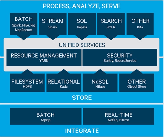
Cloudera provides a scalable, flexible, integrated platform that makes it easy to manage rapidly increasing volumes and varieties of data in any enterprise. Industry-leading Cloudera products and solutions enable enterprises to deploy and manage Apache Hadoop and related projects, manipulate and analyze data, and keep that data secure and protected.
Cloudera provides the following products and tools:
· CDH—The Cloudera distribution of Apache Hadoop and other related open-source projects, including Spark. CDH also provides security and integration with numerous hardware and software solutions.
· Apache Spark—An integrated part of CDH supported with Cloudera Enterprise, Spark is an open standard for flexible in-memory data processing for batch, real-time, and advanced analytics. Via one platform, Cloudera is committed to adopting Spark as the default data execution engine for analytic workloads.
· Cloudera Manager—A sophisticated application used to deploy, manage, monitor, and diagnose issues with CDH deployments. Cloudera Manager provides the Admin Console, a web-based user interface that makes administration of any enterprise data simple and straightforward. It also includes the Cloudera Manager API, which can be used to obtain cluster health information and metrics, as well as configure Cloudera Manager.
· Cloudera Navigator—An end-to-end data management tool for the CDH platform. Cloudera Navigator enables administrators, data managers, and analysts to explore the large amounts of data in Hadoop. The robust auditing, data management, lineage management, and life cycle management in Cloudera Navigator allow enterprises to adhere to stringent compliance and regulatory requirements.
Apache Spark
Apache Spark is a fast and general-purpose engine for large-scale data processing. By adding Apache Spark to the Hadoop deployment and analysis platform, and running it all on Cisco UCS Integrated Infrastructure for Big Data and Analytics, customers can accelerate streaming, interactive queries, machine learning, and batch workloads, and offer their user’s experiences that deliver more insights in less time.
Traditional servers are not designed to support the massive scalability, performance, and efficiency requirements of Big Data solutions. These outdated and siloed computing solutions are difficult to integrate with network and storage resources, and are time-consuming to deploy and expensive to operate. Cisco UCS Integrated Infrastructure for Big Data and Analytics with Apache Spark takes a different approach, combining computing, networking, storage access, and management capabilities into a unified, fabric-based architecture that is optimized for Big Data workloads.
Apache Spark enhances existing Big Data environments by adding new capabilities to Hadoop or other Big Data deployments. The platform unifies a broad range of capabilities—batch processing, real-time stream processing, advanced analytic capabilities, and interactive exploration that can intelligently optimize applications. Spark’s key advantage is speed, with an advanced DAG execution engine that supports cyclic data-flow and in-memory computing. It can run programs much faster than Hadoop/Map-Reduce. Applications can be developed using built-in, high-level Apache Spark operations, or they can interact with applications like Python, R, and Scala shells, or Java. These various options allow users to quickly and easily build new applications and explore data faster.
Apache Spark delivers the rapid response that is needed by real-time interactive applications, and experimentation environments. An important factor in the solution’s performance is the way Apache Spark performs operations, most of which are done in memory. Spark provides programmers with any application interface, centered on a data structure called the resilient distributed dataset (RDD), a read-only multiset of data items distributed over a cluster of machines, that is maintained in a fault-tolerant way. Calculations are performed and results are delivered only when needed, and results can be configured to persist in memory, allowing Apache Spark to deliver a new level of computing efficiency and computation performance to Big Data deployments.
Apache Spark has a number of libraries:
· Apache Spark SQL/DataFrame API for querying structured data inside Spark programs.
· Apache Spark Streaming offers Spark’s core API that is able to perform real-time processing of streaming data, including web server log files, social media, and messaging queues.
· MLLib to take advantage of machine-learning algorithms and accelerate application performance across clusters.
· GraphX unifies ETL, performs exploratory analysis, and accelerates iterative graphical computations in a single system.
Spark runs on Hadoop, Mesos, stand alone, or in the cloud. It can access diverse data sources including HDFS, Cassandra, HBase, and S3. Spark with YARN is an optimal way to schedule and run Spark jobs on a Hadoop cluster alongside a variety of other data-processing frameworks, leveraging existing clusters using queue placement policies, and enabling security by running on Kerberos-enabled clusters. There are options for yarn-client and yarn-cluster mode, please refer to Cloudera-Spark on YARN options for further details on these options.
Some common use cases that are popular in the field with Apache Spark:
· Real-Time Actions – Anomalous behaviors detected in real-time, and downstream actions are processed accordingly. For example; credit card transactions occurring in a different location generating actions for fraud alert, IOT sensors transmitting device failure data, etc.
· Data Enrichment – Live data is enriched with more information by joining it with cached static datasets, allowing for a more comprehensive features set in real-time.
· Exploratory Analytics – Events related to a specific time-window can be grouped together and analyzed. This sample data can be used by Data Scientists to update machine-learning models using tools like Python, etc. within Spark.
· Streaming Data with Analytics – The same code for streaming analytic operations can be used for batch, to compute over both the stream and historical data. This reduces moving parts and helps increase the productivity, consistency, and maintainability of analytic procedures. Spark is compatible with the rest of the streaming data ecosystem, supporting data sources including Flume, Kafka, ZeroMQ, and HDFS.
Spark Streaming
Spark Streaming brings Spark's language-integrated API to stream processing. The API is provided in Java, Scala, and Python. Spark’s single execution engine, and unified programming model for batch and streaming, lead to some unique benefits over other traditional streaming systems.
· Fast recovery from failures and stragglers.
· Better load balancing and resource usage.
· Combining streaming data with static datasets and interactive queries.
· Native integration with advanced processing libraries (SQL, machine learning, graph processing).
In Spark Streaming, batches of Resilient Distributed Datasets (RDDs) are passed to Spark Streaming, which processes these batches using the Spark Engine and returns a processed stream of batches. This processed stream can be written to the file system. Spark Streaming allows stateful computations, maintaining a state based on data coming in a stream. It also allows window operations (i.e., allows the developer to specify a time frame, and perform operations on the data flowing in that time window. The window has a sliding interval, which is the time interval of updating the window
Each batch of data is a Resilient Distributed Dataset (RDD), which is the basic abstraction of a fault-tolerant dataset in Spark. This common representation allows batch and streaming workloads to interoperate seamlessly. Users can apply arbitrary Spark functions on each batch of streaming data: for example, it’s easy to join a DStream (key programming abstraction in Spark Streaming) with a precomputed static dataset (such as an RDD). Spark interoperability extends to rich libraries like MLlib (machine learning), SQL, and DataFrames.
Machine learning models generated offline with MLlib can be applied on streaming data. Fault tolerance in Spark Streaming is similar to fault tolerance in Spark. Like RDD partitions, DStream data is recomputed in case of a failure. The raw input is replicated in memory across the cluster. In case of a node failure, the data can be reproduced using the lineage. Spark Streaming is a streaming platform and allows reaching sub-second latency. The processing capability scales linearly with the size of the cluster; hence it is being used in production by many organizations.
Spark SQL
Spark SQL allows users to query structured data inside Spark programs, using either SQL or DataFrame API. DataFrames and SQL provide a common way to access a variety of data sources, including Hive, Avro, Parquet, ORC, JSON, and JDBC. Spark SQL brings native support for SQL to Spark and streamlines the process of querying data stored both in RDDs and in external sources. Spark SQL conveniently blurs the lines between RDDs and relational tables.
Spark SQL provides, a programming abstraction DataFrame that acts as distributed SQL query engine; additional to the data sources API, Spark SQL now makes it easier to compute over structured data stored in a wide variety of formats, including Parquet, JSON, and Apache Avro library; a built-in JDBC server makes it easy to connect to the structured data stored in relational database tables and perform Big Data analytics using the traditional BI tools.
Spark SQL includes a new optimization framework (Catalyst), columnar storage, and code generation to make queries fast. Catalyst is based on functional programming constructs in Scala. Catalyst’s extensible design makes it easy to add new optimization techniques and features to Spark SQL, especially for the purpose of tackling various problems we were seeing with Big Data (e.g., semi structured data and advanced analytics). Also enables external developers to extend the optimizer — for example, by adding data source specific rules that can push filtering or aggregation into external storage systems, or support for new data types. Catalyst supports both rule-based and cost-based optimization. Catalyst offers several public extension points, including external data sources and user-defined types.
Spark SQL scales to thousands of nodes and multi hour queries using the Spark engine, which provides full mid-query fault tolerance. Spark SQL is a powerful library that non-technical team members like Business and Data Analysts can use to run data analytics in their organizations.
![]() Note: Avro has some limitations with SparkSQL; please refer to documentation here for further details. http://www.cloudera.com/documentation/enterprise/release-notes/topics/cdh_rn_spark_ki.html
Note: Avro has some limitations with SparkSQL; please refer to documentation here for further details. http://www.cloudera.com/documentation/enterprise/release-notes/topics/cdh_rn_spark_ki.html
Apache Kafka
Apache Kafka is a distributed publish-subscribe messaging system that is designed to be fast, scalable and durable. Kafka maintains feeds of messages in topics. Producers write data to topics and consumers read from topics. Since Kafka is a distributed system, topics are partitioned and replicated across multiple nodes. Kafka is designed to allow a single cluster to serve as the central data backbone for a large organization. It can be elastically and transparently expanded without downtime. Data streams are partitioned and spread over a cluster of machines to allow data streams larger than the capability of any single machine and to allow clusters of coordinated consumers.
· Messages are simply byte arrays and developers can use them to store any object in any format, with String, JSON, and Avro the most common. It is possible to attach a key to each message, in which case the producer guarantees that all messages with the same key will arrive to the same partition.
· Messages are persisted on disk and replicated within the cluster to prevent data loss. Each broker can handle terabytes of messages without performance impact. When consuming from a topic, it is possible to configure a consumer group with multiple consumers. Each consumer in a consumer group will read messages from a unique subset of partitions in each topic they subscribe to, so each message is delivered to one consumer in the group, and all messages with the same key arrive at the same consumer.
What makes Kafka unique is that Kafka treats each topic partition as a log (an ordered set of messages). Each message in a partition is assigned a unique offset. Kafka does not attempt to track, which messages were read by each consumer and only retain unread messages; rather, Kafka retains all messages for a set amount of time, and consumers are responsible to track their location in each log. Consequently, Kafka can support a large number of consumers and retain large amounts of data with very little overhead.
Kafka is very popular is a number of use cases like
· Website activity tracking— The web application sends events such as page views and searches Kafka, where they become available for real-time processing, dashboards and offline analytics in Hadoop.
· Operational metrics— Alerting and reporting on operational metrics. One particularly fun example is having Kafka producers and consumers occasionally publish their message counts to a special Kafka topic; a service can be used to compare counts and alert if data loss occurs.
· Log aggregation— Kafka can be used across an organization to collect logs from multiple services and make them available in standard format to multiple consumers, including Hadoop and Apache Solr.
· Stream processing— A framework such as Spark Streaming reads data from a topic, processes it and writes processed data to a new topic where it becomes available for users and applications. Kafka’s strong durability is also very useful in the context of stream processing.
Kafka allows clients to choose synchronous or asynchronous replications. In the former case message is acknowledged only after it reaches multiple replicas, in the latter case a message to be published is acknowledged as soon as it reaches one replica. The purpose of adding replication in Kafka is for stronger durability and higher availability. Details on how to configure the replicas are captured later in this document.
Apache Flume
Flume is a distributed, reliable, and available service for efficiently collecting, aggregating, and moving large amounts of log data. It has a simple and flexible architecture based on streaming data flows. It is robust and fault tolerant with tunable reliability mechanisms and many failover and recovery mechanisms. It uses a simple extensible data model that allows for online analytic application.
A Flume event is defined as a unit of data flow having a byte payload and an optional set of string attributes. A Flume agent is a (JVM) process that hosts the components through which events flow an external source to the next destination (hop). A Flume source consumes events delivered to it by an external source like a web server. The external source sends events to Flume in a format that is recognized by the target Flume source. For example, an Avro Flume source can be used to receive Avro events from Avro clients or other Flume agents in the flow that send events from an Avro sink. When a Flume source receives an event, it stores it into one or more channels. The channel is a passive store that keeps the event until it’s consumed by a Flume sink. The file channel is one example – it is backed by the local file system. The sink removes the event from the channel and puts it into an external repository like HDFS (via Flume HDFS sink) or forwards it to the Flume source of the next Flume agent (next hop) in the flow. The source and sink within the given agent run asynchronously with the events staged in the channel. Flume allows a user to build multi-hop flows where events travel through multiple agents before reaching the final destination. It also allows fan-in and fan-out flows, contextual routing and backup routes (fail-over) for failed hops.
Below are some popular features of Flume.
· Stream Data– Ingest streaming data from multiple sources into Hadoop for storage and analysis.
· Throttle data from incoming channels– Buffer the storage platform from spikes when rate of incoming data exceeds the rate at which data can be consumed.
· Scale horizontally– Ingest new data streams and additional volumes as needed.
Kafka/Flume Comparison
There is significant overlap in the functions of Flume and Kafka. Here are some considerations when evaluating the two systems.
· Kafka is a distributed messaging system and it can have many producers and many consumers sharing multiple topics but there are some limitations on message size. Flume is a special-purpose tool designed to send data to HDFS and HBase. It has specific optimizations for HDFS and it integrates seamlessly with Hadoop’s security.
· Flume has many built-in sources and sinks. Use Flume if the existing Flume sources and sinks match the requirements and there is a preference for a system that can be set up without any development.
· Flume can process data in-flight using interceptors. These can be very useful for data masking or filtering. Kafka requires an external stream processing system for that.
· Both Kafka and Flume are reliable systems that with proper configuration can guarantee zero data loss. However, Flume does not replicate events. Use Kafka if there is a need for an ingest pipeline with very high availability.
· Flume and Kafka can work quite well together. If the design requires streaming data from Kafka to Hadoop, using a Flume agent with Kafka source to read the data makes sense.
Requirements
This CVD describes architecture and deployment procedures for Cloudera (CDH 5.7.0) on a 64 Cisco UCS C240 M4SX node cluster based on Cisco UCS Integrated Infrastructure for Big Data and Analytics. The solution goes into detail configuring CDH 5.7.0 on the infrastructure. In addition it also details the configuration for Apache Spark for various use cases.
The Performance cluster configuration consists of the following:
· Two Cisco UCS 6296UP Fabric Interconnects
· 64 UCS C240 M4 Rack-Mount servers (16 per rack)
· Four Cisco R42610 standard racks
· Eight Vertical Power distribution units (PDUs) (Country Specific)
Rack and PDU Configuration
Each rack consists of two vertical PDUs. The master rack consists of two Cisco UCS 6296UP Fabric Interconnects, sixteen Cisco UCS C240 M4 Servers connected to each of the vertical PDUs for redundancy; thereby, ensuring availability during power source failure. The expansion racks consists of sixteen Cisco UCS C240 M4 Servers connected to each of the vertical PDUs for redundancy; thereby, ensuring availability during power source failure, similar to the master rack.
![]() Note: Please contact your Cisco representative for country specific information.
Note: Please contact your Cisco representative for country specific information.
Error! Reference source not found. describes the rack configurations of rack 1 (master rack) and racks 2-4 (expansion racks).
Table 4 Rack 1 (Master Rack) Racks 2-4 (Expansion Racks)
| Cisco |
Master Rack |
Cisco |
Expansion Rack |
| 42URack |
|
42URack |
|
| 42 |
Cisco UCS FI 6296UP |
42 |
Unused |
| 41 |
41 |
Unused |
|
| 40 |
Cisco UCS FI 6296UP |
40 |
Unused |
| 39 |
39 |
Unused |
|
| 38 |
Unused |
38 |
Unused |
| 37 |
Unused |
37 |
Unused |
| 36 |
Unused |
36 |
Unused |
| 35 |
35 |
Unused |
|
| 34 |
Unused
|
34 |
Unused |
| 33 |
33 |
Unused |
|
| 32 |
Cisco UCS C240 M4 |
32 |
Cisco UCS C240 M4 |
| 31 |
31 |
|
|
| 30 |
Cisco UCS C240 M4 |
30 |
Cisco UCS C240 M4 |
| 29 |
29 |
|
|
| 8 |
Cisco UCS C240 M4 |
28 |
Cisco UCS C240 M4 |
| 27 |
27 |
|
|
| 26 |
Cisco UCS C240 M4 |
26 |
Cisco UCS C240 M4 |
| 25 |
25 |
|
|
| 24 |
Cisco UCS C240 M4 |
24 |
Cisco UCS C240 M4 |
| 23 |
23 |
|
|
| 22 |
Cisco UCS C240 M4 |
22 |
Cisco UCS C240 M4 |
| 21 |
21 |
|
|
| 20 |
Cisco UCS C240 M4 |
20 |
Cisco UCS C240 M4 |
| 19 |
19 |
|
|
| 18 |
Cisco UCS C240 M4 |
18 |
Cisco UCS C240 M4 |
| 17 |
17 |
Cisco UCS C240 M4 |
|
| 16 |
Cisco UCS C240 M4 |
16 |
|
| 15 |
15 |
|
|
| 14 |
Cisco UCS C240 M4 |
14 |
Cisco UCS C240 M4 |
| 13 |
13 |
|
|
| 12 |
Cisco UCS C240 M4 |
12 |
Cisco UCS C240 M4 |
| 11 |
11 |
|
|
| 10 |
Cisco UCS C240 M4 |
10 |
Cisco UCS C240 M4 |
| 9 |
9 |
|
|
| 8 |
Cisco UCS C240 M4 |
8 |
Cisco UCS C240 M4 |
| 7 |
7 |
|
|
| 6 |
Cisco UCS C240 M4 |
6 |
Cisco UCS C240 M4 |
| 5 |
5 |
|
|
| 4 |
Cisco UCS C240 M4 |
4 |
Cisco UCS C240 M4 |
| 3 |
3 |
|
|
| 2 |
Cisco UCS C240 M4 |
2 |
Cisco UCS C240 M4 |
| 1 |
1 |
|
|
|
|
|
|
|
Port Configuration on Fabric Interconnects
| Port Type |
Port Number |
| Network |
1 |
| Server |
2 to 65 |
Server Configuration and Cabling for C240M4
The C240 M4 rack server is equipped with Intel Xeon E5-2680 v4 processors, 256 GB of memory, Cisco UCS Virtual Interface Card 1227, Cisco 12-Gbps SAS Modular Raid Controller with 2-GB FBWC, 24 1.8-TB 10K SFF SAS drives, 2 240-GB SATA SSD for Boot.
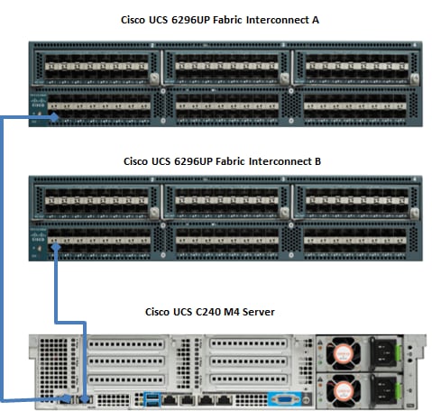
Figure 12 illustrates the port connectivity between the Fabric Interconnect, and Cisco UCS C240 M4 server. Sixteen Cisco UCS C240 M4 servers are used in Master rack configurations.
Figure 12 Fabric Topology for C240 M4
For more information on physical connectivity and single-wire management see:
For more information on physical connectivity illustrations and cluster setup, see:
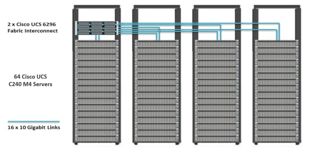
Figure 13 depicts a 64-node cluster. Every rack has 16 Cisco UCS C240 M4 servers. Each link in the figure represents 16 x 10 Gigabit Ethernet link from each of the 16 servers connecting to a Fabric Interconnect as a Direct Connect. Every server is connected to both Fabric Interconnect represented with dual link.
Figure 13 64 Nodes Cluster Configuration
Software Distributions and Versions
The required software distribution versions are listed below.
Cloudera (CDH 5.7.0)
The Cloudera Distribution for Apache Hadoop version used is 5.7.0. For more information visit www.cloudera.com.
Red Hat Enterprise Linux (RHEL)
The operating system supported is Red Hat Enterprise Linux 7.2. For more information visit http://www.redhat.com.
Software Versions
The software versions tested and validated in this document are shown in Table 5 .
| Layer |
Component |
Version or Release |
| Compute |
Cisco UCS C240-M4 |
C240M4.2.0.10c |
| Network |
Cisco UCS 6296UP |
UCS 3.1(1g) A |
| Cisco UCS VIC1227 Firmware |
4.1.1(d) |
|
| Cisco UCS VIC1227 Driver |
2.3.0.20 |
|
| Storage |
LSI SAS 3108 |
24.9.1-0011 |
|
|
LSI MegaRAID SAS Driver |
06.810.10.00 |
| Software |
Red Hat Enterprise Linux Server |
7.2 (x86_64) |
| Cisco UCS Manager |
3.1(1g) |
|
| CDH |
5.7.0 |
![]() The latest drivers can be downloaded from the link below:
The latest drivers can be downloaded from the link below:
https://software.cisco.com/download/release.html?mdfid=283862063&flowid=25886&softwareid=283853158&release=1.5.7d&relind=AVAILABLE&rellifecycle=&reltype=latest
![]() The Latest Supported RAID controller Driver is already included with the RHEL 7.2 operating system
The Latest Supported RAID controller Driver is already included with the RHEL 7.2 operating system
![]() C240 M4 Rack Servers with Broadwell (E5 -2600 v4) CPUs are supported from UCS firmware 3.1(1g) onwards.
C240 M4 Rack Servers with Broadwell (E5 -2600 v4) CPUs are supported from UCS firmware 3.1(1g) onwards.
Fabric Configuration
This section provides details for configuring a fully redundant, highly available Cisco UCS 6296 fabric configuration.
· Initial setup of the Fabric Interconnect A and B.
· Connect to UCS Manager using virtual IP address of using the web browser.
· Launch UCS Manager.
· Enable server, uplink and appliance ports.
· Start discovery process.
· Create pools and polices for service profile template.
· Create Service Profile template and 64 Service profiles.
· Associate Service Profiles to servers.
Performing Initial Setup of Cisco UCS 6296 Fabric Interconnects
This section describes the initial setup of the Cisco UCS 6296 Fabric Interconnects A and B.
Configure Fabric Interconnect A
1. Connect to the console port on the first Cisco UCS 6296 Fabric Interconnect.
2. At the prompt to enter the configuration method, enter console to continue.
3. If asked to either perform a new setup or restore from backup, enter setup to continue.
4. Enter y to continue to set up a new Fabric Interconnect.
5. Enter y to enforce strong passwords.
6. Enter the password for the admin user.
7. Enter the same password again to confirm the password for the admin user.
8. When asked if this fabric interconnect is part of a cluster, answer y to continue.
9. Enter A for the switch fabric.
10. Enter the cluster name for the system name.
11. Enter the Mgmt0 IPv4 address.
12. Enter the Mgmt0 IPv4 netmask.
13. Enter the IPv4 address of the default gateway.
14. Enter the cluster IPv4 address.
15. To configure DNS, answer y.
16. Enter the DNS IPv4 address.
17. Answer y to set up the default domain name.
18. Enter the default domain name.
19. Review the settings that were printed to the console, and if they are correct, answer yes to save the configuration.
20. Wait for the login prompt to make sure the configuration has been saved.
Configure Fabric Interconnect B
1. Connect to the console port on the second Cisco UCS 6296 Fabric Interconnect.
2. When prompted to enter the configuration method, enter console to continue.
3. The installer detects the presence of the partner Fabric Interconnect and adds this fabric interconnect to the cluster. Enter y to continue the installation.
4. Enter the admin password that was configured for the first Fabric Interconnect.
5. Enter the Mgmt0 IPv4 address.
6. Answer yes to save the configuration.
7. Wait for the login prompt to confirm that the configuration has been saved.
For more information on configuring Cisco UCS 6200 Series Fabric Interconnect, see: http://www.cisco.com/en/US/docs/unified_computing/ucs/sw/gui/config/guide/2.0/b_UCSM_GUI_Configuration_Guide_2_0_chapter_0100.html.
Logging Into Cisco UCS Manager
To login to Cisco UCS Manager, complete the following steps:
1. Open a Web browser and navigate to the Cisco UCS 6296 Fabric Interconnect cluster address.
2. Click the Launch link to download the Cisco UCS Manager software.
3. If prompted to accept security certificates, accept as necessary.
4. When prompted, enter admin for the username and enter the administrative password.
5. Click Login to log in to the Cisco UCS Manager.
Upgrading UCSM Software to Version 3.1(1g)
This document assumes the use of UCS 3.1(1g) Refer to Cisco UCS 3.1 Release (upgrade the Cisco UCS Manager software and UCS 6296 Fabric Interconnect software to version 3.1(1g). Also, make sure the UCS C-Series version 3.1(1g) software bundles is installed on the Fabric Interconnects.
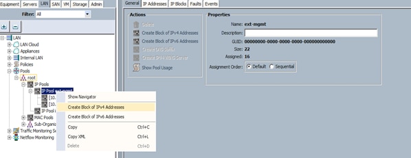
Adding a Block of IP Addresses for KVM Access
These steps provide details for creating a block of KVM IP addresses for server access in the Cisco UCS environment.
1. Select the LAN tab at the top of the left window.
2. Select Pools > IpPools > Ip Pool ext-mgmt.
3. Right-click IP Pool ext-mgmt.
4. Select Create Block of IPv4 Addresses.
Figure 14 Adding a Block of IPv4 Addresses for KVM Access Part 1
5. Enter the starting IP address of the block and number of IPs needed, as well as the subnet and gateway information.
Figure 15 Adding Block of IPv4 Addresses for KVM Access Part 2
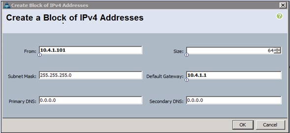
6. Click OK to create the IP block.
7. Click OK in the message box.
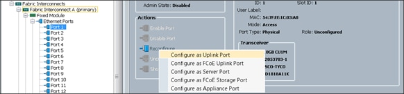
Enabling Uplink Ports
To enable uplinks ports, complete the following steps:
1. Select the Equipment tab on the top left of the window.
2. Select Equipment > Fabric Interconnects > Fabric Interconnect A (primary) > Fixed Module.
3. Expand the Unconfigured Ethernet Ports section.
4. Select port 1 that is connected to the uplink switch, right-click, then select Reconfigure > Configure as Uplink Port.
5. Select Show Interface and select 10GB for Uplink Connection.
6. A pop-up window appears to confirm your selection. Click Yes then OK to continue.
7. Select Equipment > Fabric Interconnects > Fabric Interconnect B (subordinate) > Fixed Module.
8. Expand the Unconfigured Ethernet Ports section.
9. Select port number 1, which is connected to the uplink switch, right-click, then select Reconfigure > Configure as Uplink Port.
10. Select Show Interface and select 10GB for Uplink Connection.
11. A pop-up window appears to confirm your selection. Click Yes then OK to continue.
Figure 16 Enabling Uplink Ports
Configuring VLANs
VLANs are configured as in shown in Table 6 .
| VLAN |
NIC Port |
Function |
| VLAN19 |
eth0 |
Data |
The NIC will carry the data traffic from VLAN19. A single vNIC is used in this configuration and the Fabric Failover feature in Fabric Interconnects will take care of any physical port down issues. It will be a seamless transition from an application perspective.
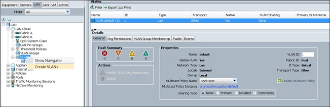
To configure VLANs in the Cisco UCS Manager GUI, complete the following steps:
1. Select the LAN tab in the left pane in the UCSM GUI.
2. Select LAN > LAN Cloud > VLANs.
3. Right-click the VLANs under the root organization.
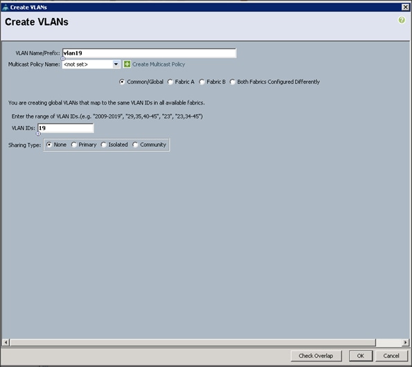
4. Select Create VLANs to create the VLAN.
Figure 17 Creating a VLAN
5. Enter vlan19 for the VLAN Name.
6. Keep multicast policy as <not set>.
7. Select Common/Global for vlan19.
8. Enter 19 in the VLAN IDs field for the Create VLAN IDs.
9. Click OK and then, click Finish.
10. Click OK in the success message box.
Figure 18: Creating VLAN for Data
11. Click OK and then, click Finish.
Enabling Server Ports
To enable server ports, complete the following steps:
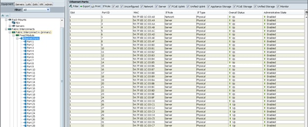
1. Select the Equipment tab on the top left of the window.
2. Select Equipment > Fabric Interconnects > Fabric Interconnect A (primary) > Fixed Module.
3. Expand the Unconfigured Ethernet Ports section.
4. Select all the ports that are connected to the Servers right-click them, and select Reconfigure > Configure as a Server Port.
5. A pop-up window appears to confirm your selection. Click Yes then OK to continue.
6. Select Equipment > Fabric Interconnects > Fabric Interconnect B (subordinate) > Fixed Module.
7. Expand the Unconfigured Ethernet Ports section.
8. Select all the ports that are connected to the Servers right-click them, and select Reconfigure > Configure as a Server Port.
9. A pop-up window appears to confirm your selection. Click Yes, then OK to continue.
Figure 18 Enabling Server Ports
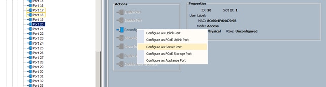
After the Server Discovery, Port 1 will be a Network Port and 2-65 will be Server Ports.
Noy
Creating Pools for Service Profile Templates
Creating an Organization
Organizations are used as a means to arrange and restrict access to various groups within the IT organization, thereby enabling multi-tenancy of the compute resources. This document does not assume the use of Organizations; however the necessary steps are provided for future reference.
To configure an organization within the Cisco UCS Manager GUI, complete the following steps:
1. Click New on the top left corner in the right pane in the UCS Manager GUI.
2. Select Create Organization from the options
3. Enter a name for the organization.
4. (Optional) Enter a description for the organization.
5. Click OK.
6. Click OK in the success message box.
Creating MAC Address Pools
To create MAC address pools, complete the following steps:
1. Select the LAN tab on the left of the window.
2. Select Pools > root.
3. Right-click MAC Pools under the root organization.
4. Select Create MAC Pool to create the MAC address pool. Enter ucs for the name of the MAC pool.
5. (Optional) Enter a description of the MAC pool.
6. Select Assignment Order Sequential.
7. Click Next.
8. Click Add.
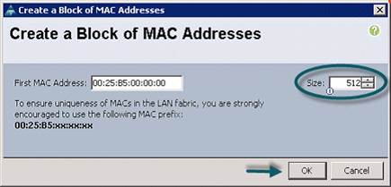
9. Specify a starting MAC address.
10. Specify a size of the MAC address pool, which is sufficient to support the available server resources.
11. Click OK.
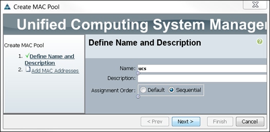
Figure 19 Specifying first MAC Address and Size
12. Click Finish.
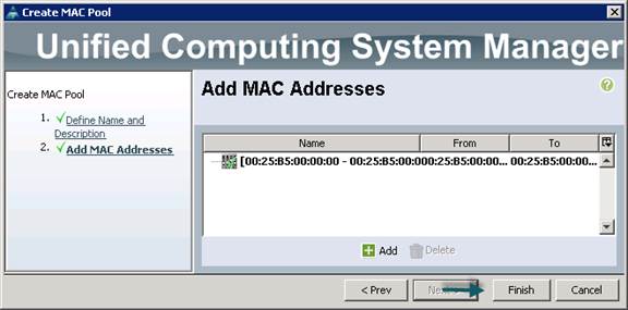
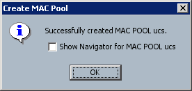
13. When the message box displays, click OK.
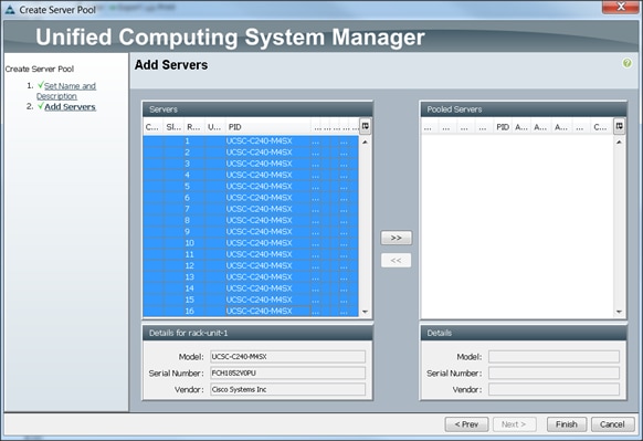
Creating a Server Pool
A server pool contains a set of servers. These servers typically share the same characteristics. Those characteristics can be their location in the chassis, or an attribute such as server type, amount of memory, local storage, type of CPU, or local drive configuration. You can manually assign a server to a server pool, or use server pool policies and server pool policy qualifications to automate the assignment
To configure the server pool within the Cisco UCS Manager GUI, complete the following steps:
1. Select the Servers tab in the left pane in the UCS Manager GUI.
2. Select Pools > root.
3. Right-click the Server Pools.
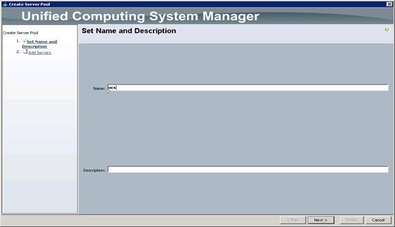
4. Select Create Server Pool.
5. Enter your required name (ucs) for the Server Pool in the name text box.
6. (Optional) enter a description for the organization.
7. Click Next > to add the servers.
8. Select all the Cisco UCS C240M4SX servers to be added to the server pool that was previously created (ucs), then Click >> to add them to the pool.
9. Click Finish.
10. Click OK and then click Finish.
Creating Policies for Service Profile Templates
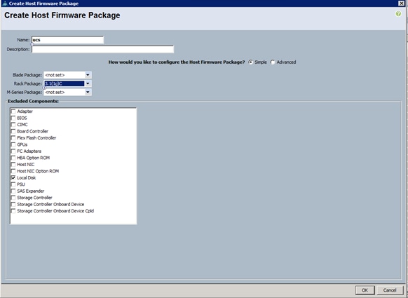
Creating Host Firmware Package Policy
Firmware management policies allow the administrator to select the corresponding packages for a given server configuration. These include adapters, BIOS, board controllers, FC adapters, HBA options, and storage controller properties as applicable.
To create a firmware management policy for a given server configuration using the Cisco UCS Manager GUI, complete the following steps:
1. Select the Servers tab in the left pane in the UCS Manager GUI.
2. Select Policies > root.
3. Right-click Host Firmware Packages.
4. Select Create Host Firmware Package.
5. Enter the required Host Firmware package name (ucs).
6. Select Simple radio button to configure the Host Firmware package.
7. Select the appropriate Rack package that has been installed.
8. Click OK to complete creating the management firmware package
9. Click OK.
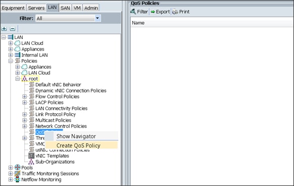
Creating QoS Policies
To create the QoS policy for a given server configuration using the Cisco UCS Manager GUI, complete the following steps:
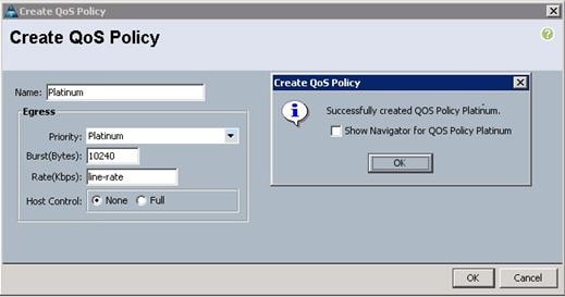
Platinum Policy
1. Select the LAN tab in the left pane in the UCS Manager GUI.
2. Select Policies > root.
3. Right-click QoS Policies.
4. Select Create QoS Policy.
5. Enter Platinum as the name of the policy.
6. Select Platinum from the drop down menu.
7. Keep the Burst(Bytes) field set to default (10240).
8. Keep the Rate(Kbps) field set to default (line-rate).
9. Keep Host Control radio button set to default (none).
10. Once the pop-up window appears, click OK to complete the creation of the Policy.
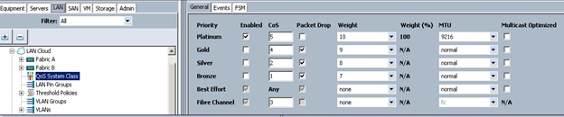
Setting Jumbo Frames
To set Jumbo frames and enable QoS, complete the following steps:
1. Select the LAN tab in the left pane in the UCSM GUI.
2. Select LAN Cloud > QoS System Class.
3. In the right pane, select the General tab
4. In the Platinum row, enter 9216 for MTU.
5. Check the Enabled Check box next to Platinum.
6. In the Best Effort row, select none for weight.
7. In the Fiber Channel row, select none for weight.
8. Click Save Changes.
9. Click OK.
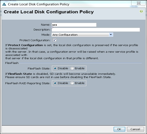
Creating the Local Disk Configuration Policy
To create local disk configuration in the Cisco UCS Manager GUI, complete the following steps:
1. Select the Servers tab on the left pane in the UCS Manager GUI.
2. Go to Policies > root.
3. Right-click Local Disk Config Policies.
4. Select Create Local Disk Configuration Policy.
5. Enter ucs as the local disk configuration policy name.
6. Change the Mode to Any Configuration. Check the Protect Configuration box.
7. Keep the FlexFlash State field as default (Disable).
8. Keep the FlexFlash RAID Reporting State field as default (Disable).
9. Click OK to complete the creation of the Local Disk Configuration Policy.
10. Click OK.
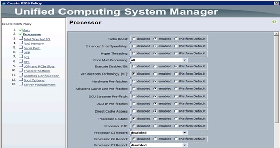
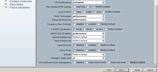
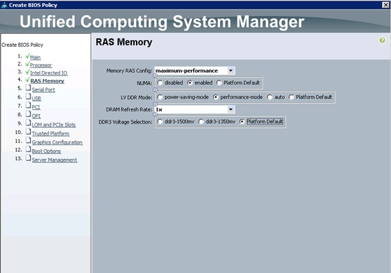
Creating Server BIOS Policy
The BIOS policy feature in Cisco UCS automates the BIOS configuration process. The traditional method of setting the BIOS is manually, and is often error-prone. By creating a BIOS policy and assigning the policy to a server or group of servers, can enable transparency within the BIOS settings configuration.
![]() Note: BIOS settings can have a significant performance impact, depending on the workload and the applications. The BIOS settings listed in this section is for configurations optimized for best performance which can be adjusted based on the application, performance, and energy efficiency requirements.
Note: BIOS settings can have a significant performance impact, depending on the workload and the applications. The BIOS settings listed in this section is for configurations optimized for best performance which can be adjusted based on the application, performance, and energy efficiency requirements.
To create a server BIOS policy using the Cisco UCS Manager GUI, complete the following steps:
1. Select the Servers tab in the left pane in the UCS Manager GUI.
2. Select Policies > root.
3. Right-click BIOS Policies.
4. Select Create BIOS Policy.
5. Enter your preferred BIOS policy name (ucs).
6. Change the BIOS settings as shown in the following figures.
7. Only changes that need to be made are in the Processor and RAS Memory settings.
Creating the Boot Policy
To create boot policies within the Cisco UCS Manager GUI, complete the following steps:
1. Select the Servers tab in the left pane in the UCS Manager GUI.
2. Select Policies > root.
3. Right-click the Boot Policies.
4. Select Create Boot Policy.
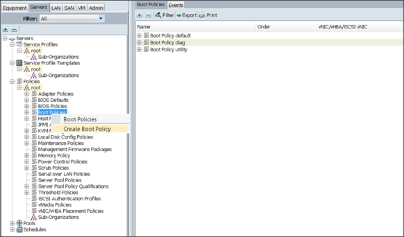
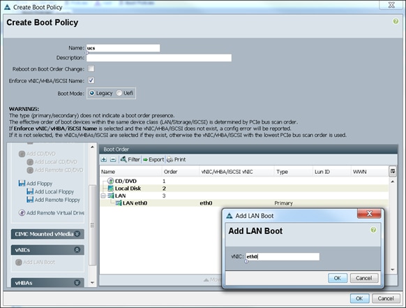
5. Enter ucs as the boot policy name.
6. (Optional) enter a description for the boot policy.
7. Keep the Reboot on Boot Order Change check box unchecked.
8. Keep Enforce vNIC/vHBA/iSCSI Name check box checked.
9. Keep Boot Mode Default (Legacy).
10. Expand Local Devices > Add CD/DVD and select Add Local CD/DVD.
11. Expand Local Devices and select Add Local Disk.
12. Expand vNICs and select Add LAN Boot and enter eth0.
13. Click OK to add the Boot Policy.
14. Click OK.
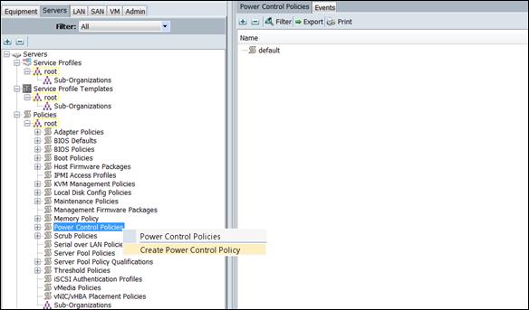
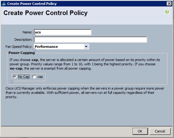
Creating Power Control Policy
To create Power Control policies within the Cisco UCS Manager GUI, complete the following steps:
1. Select the Servers tab in the left pane in the UCS Manager GUI.
2. Select Policies > root.
3. Right-click the Power Control Policies.
4. Select Create Power Control Policy.
5. Enter ucs as the Power Control policy name.
6. (Optional) enter a description for the boot policy.
7. Select Performance for Fan Speed Policy.
8. Select No cap for Power Capping selection.
9. Click OK to create the Power Control Policy.
10. Click OK.
Creating a Service Profile Template
To create a Service Profile Template, complete the following steps:
1. Select the Servers tab in the left pane in the UCSM GUI.
2. Right-click Service Profile Templates.
3. Select Create Service Profile Template.
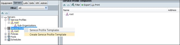
The Create Service Profile Template window appears.
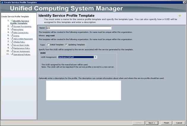
To identify the service profile template, complete the following steps:
4. Name the service profile template as ucs. Select the Updating Template radio button.
5. In the UUID section, select Hardware Default as the UUID pool.
6. Click Next to continue to the next section.
Configuring the Storage Provisioning for the Template
To configure storage policies, complete the following steps:
1. Go to the Local Disk Configuration Policy tab, and select ucs for the Local Storage.
2. Click Next to continue to the next section.
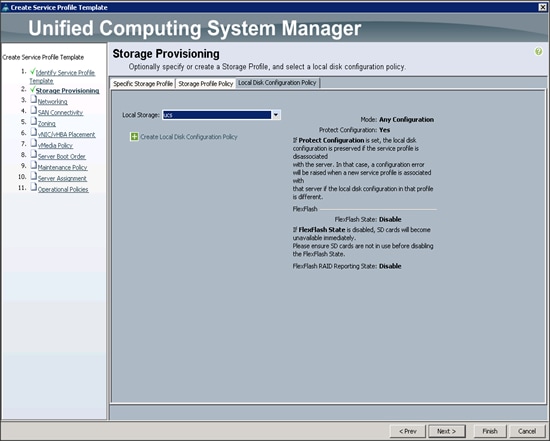
3. Click Next once the Networking window appears to go to the next section.
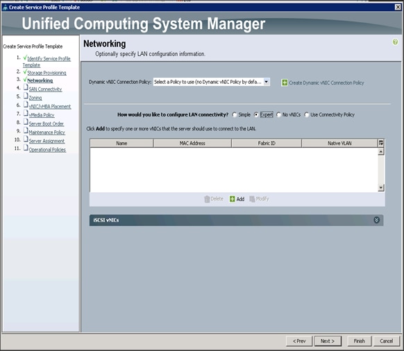
Configuring Network Settings for the Template
1. Keep the Dynamic vNIC Connection Policy field at the default.
2. Select Expert radio button for the option how would you like to configure LAN connectivity?
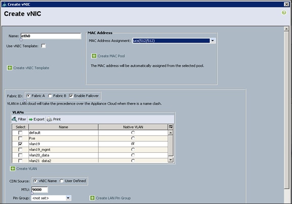
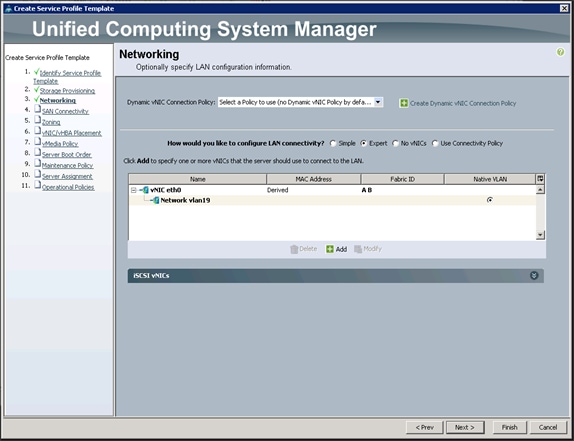
3. Click Add to add a vNIC to the template.
4. The Create vNIC window displays. Name the vNIC as eth0.
5. Select ucs in the Mac Address Assignment pool.
6. Select the Fabric A radio button and check the Enable failover check box for the Fabric ID.
7. Check the VLAN19 check box for VLANs and select the Native VLAN radio button.
8. Select MTU size as 9000.
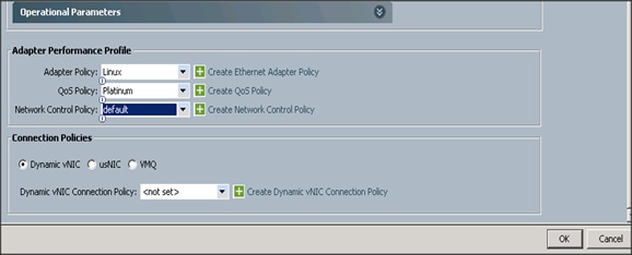
9. Select adapter policy as Linux.
10. Select QoS Policy as Platinum.
11. Keep the Network Control Policy as Default.
12. Click OK.
![]() Note: Optionally Network Bonding can be setup on the vNICs for each host for redundancy as well as for increased throughput; steps for this are captured in the Appendix 1.
Note: Optionally Network Bonding can be setup on the vNICs for each host for redundancy as well as for increased throughput; steps for this are captured in the Appendix 1.
13. Click Next to continue with SAN Connectivity.
14. Select no vHBAs for How would you like to configure SAN Connectivity?
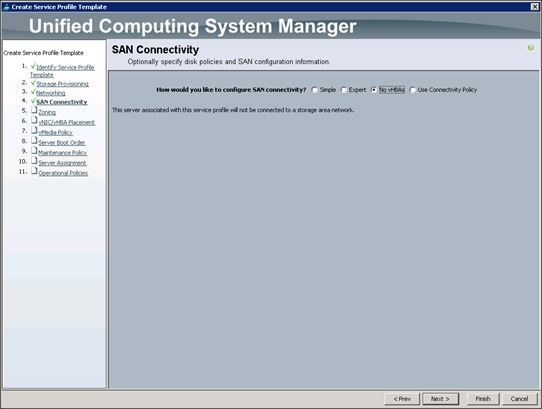
15. Click Next to continue with Zoning.
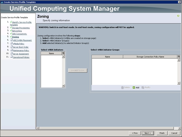
16. Click Next to continue with vNIC/vHBA placement.
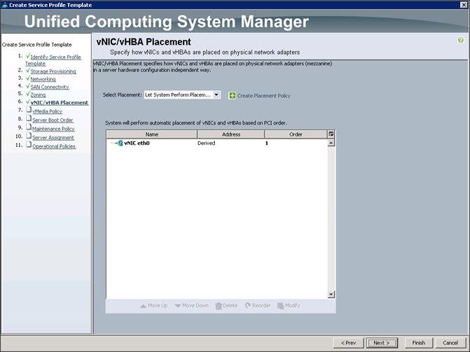
17. Click Next to configure vMedia Policy.
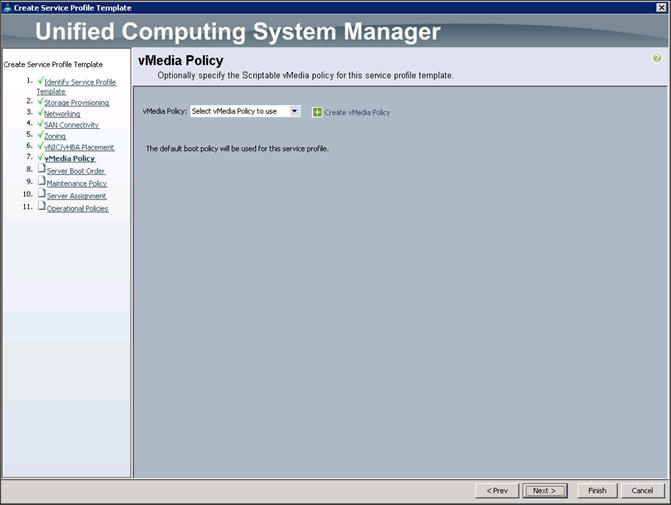
Configuring the vMedia Policy for the Template
1. Click Next once the vMedia Policy window appears to go to the next section.
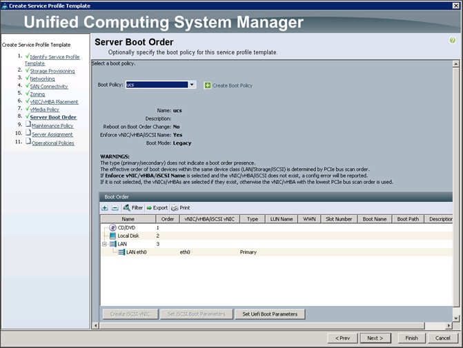
Configuring Server Boot Order for the Template
To set the boot order for the servers, complete the following steps:
1. Select ucs in the Boot Policy name field.
2. Review to make sure that all of the boot devices were created and identified.
3. Verify that the boot devices are in the correct boot sequence.
4. Click OK.
5. Click Next to continue to the next section.
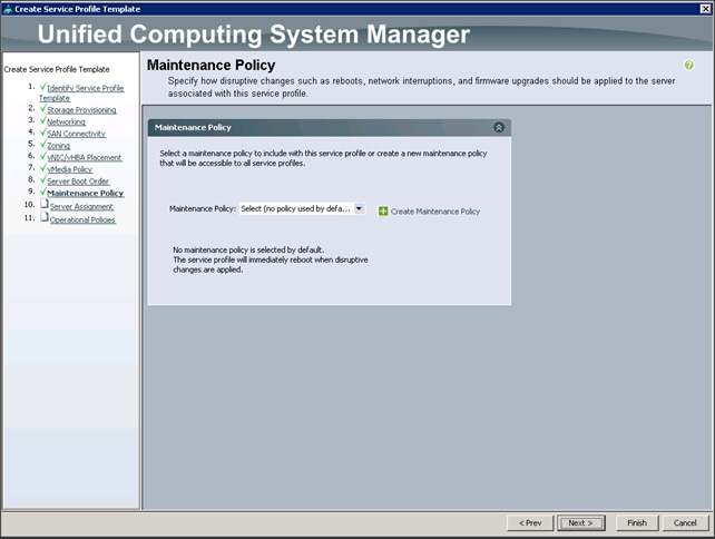
6. In the Maintenance Policy window, apply the maintenance policy.
7. Keep the Maintenance policy at no policy used by default. Click Next to continue to the next section.
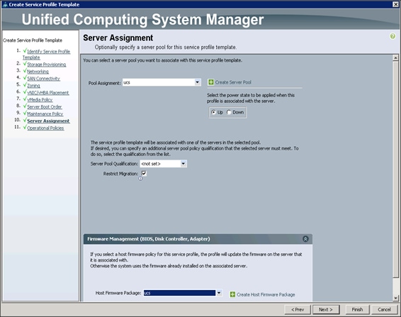
Configuring Server Assignment for the Template
In the Server Assignment window, to assign the servers to the pool, complete the following steps:
1. Select ucs for the Pool Assignment field.
2. Select the power state to be Up.
3. Keep the Server Pool Qualification field set to <not set>.
4. Check the Restrict Migration check box.
5. Select ucs in Host Firmware Package.
Configuring Operational Policies for the Template
In the Operational Policies Window, complete the following steps:
1. Select ucs in the BIOS Policy field.
2. Select ucs in the Power Control Policy field.
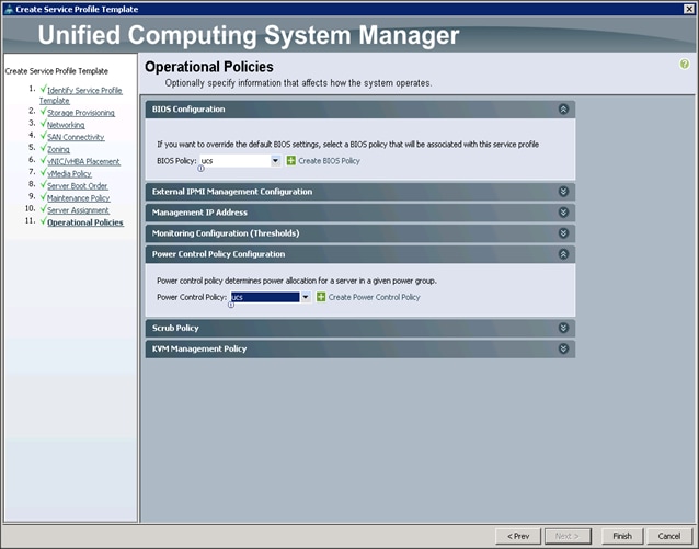
3. Click Finish to create the Service Profile template.
4. Click OK in the pop-up window to proceed.
5. Select the Servers tab in the left pane of the UCS Manager GUI.
6. Go to Service Profile Templates > root.
7. Right-click Service Profile Templates ucs.
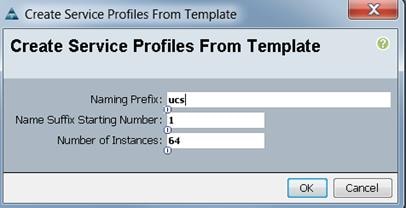
8. Select Create Service Profiles From Template.
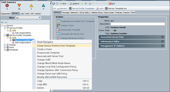
The Create Service Profiles from Template window appears.
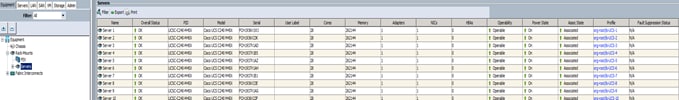
Association of the Service Profiles will take place automatically.
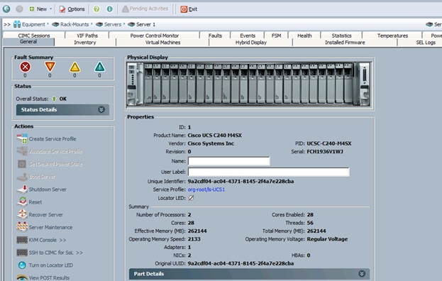
The final Cisco UCS Manager window is shown in below.
Installing Red Hat Enterprise Linux 7.2
The following section provides detailed procedures for installing Red Hat Enterprise Linux 7.2 using Software RAID (OS based Mirroring) on Cisco UCS C240 M4 servers. There are multiple ways to install the Red Hat Linux operating system. The installation procedure described in this deployment guide uses KVM console and virtual media from Cisco UCS Manager.
![]() Note: This requires RHEL 7.2 DVD/ISO for the installation
Note: This requires RHEL 7.2 DVD/ISO for the installation
To install the Red Hat Linux 7.2 operating system, complete the following steps:
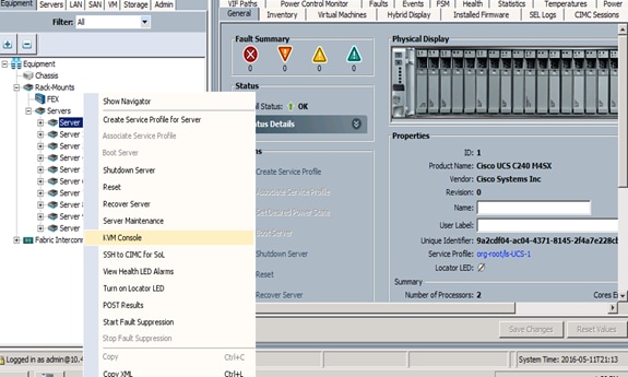
1. Log in to the Cisco UCS 6296 Fabric Interconnect and launch the Cisco UCS Manager application.
2. Select the Equipment tab.
3. In the navigation pane expand Rack-Mounts and then Servers.
4. Right click on the server and select KVM Console.
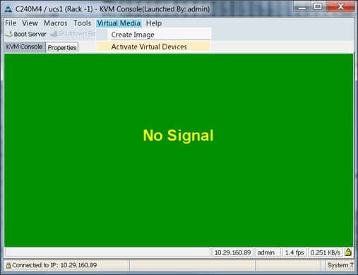
5. In the KVM window, select the Virtual Media tab.
6. Click the Activate Virtual Devices found in Virtual Media tab.
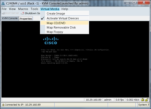
7. In the KVM window, select the Virtual Media tab and click the Map CD/DVD.
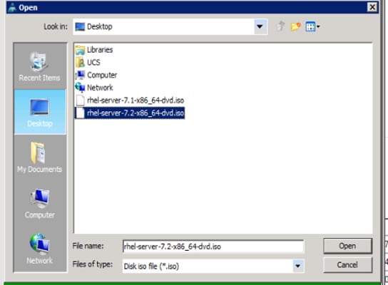
8. Browse to the Red Hat Enterprise Linux Server 7.2 installer ISO image file.
![]() Note: The Red Hat Enterprise Linux 7.2 DVD is assumed to be on the client machine.
Note: The Red Hat Enterprise Linux 7.2 DVD is assumed to be on the client machine.
9. Click Open to add the image to the list of virtual media.
10. In the KVM window, select the KVM tab to monitor during boot.
11. In the KVM window, select the Macros > Static Macros > Ctrl-Alt-Del button in the upper left corner.
12. Click OK.
13. Click OK to reboot the system.
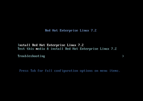
14. On reboot, the machine detects the presence of the Red Hat Enterprise Linux Server 7.2 install media.
15. Select the Install or Upgrade an Existing System.
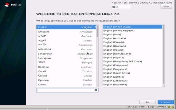
16. Skip the Media test and start the installation. Select language of installation and click Continue.
17. Select Date and time, which pops up another window as shown below:
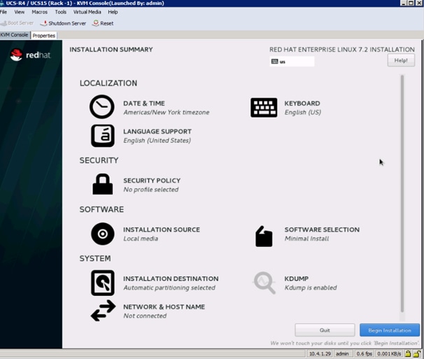
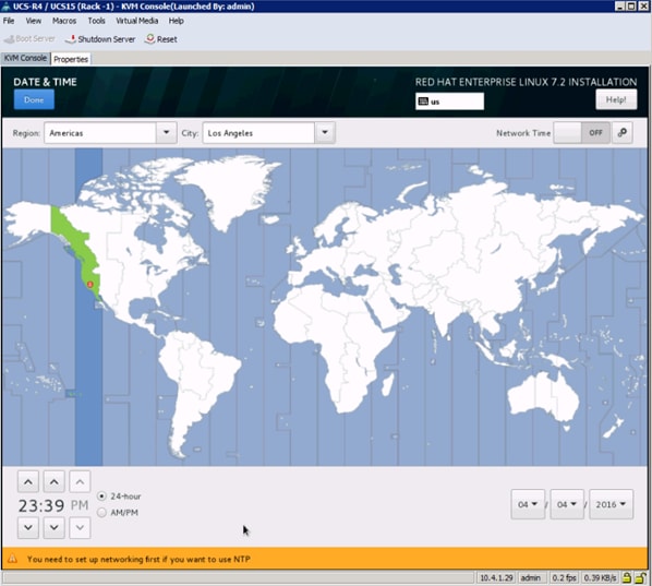
18. Select the location on the map, set the time and click Done.
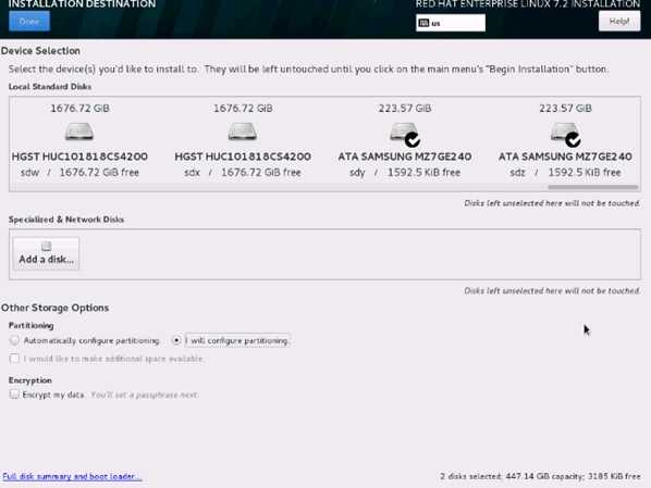
19. Click on Installation Destination.
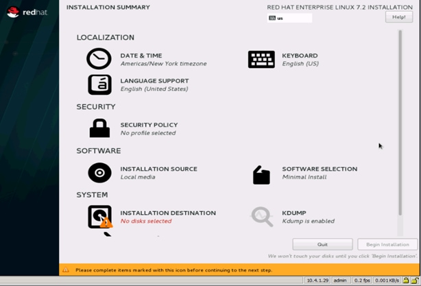
20. This opens a new window with the boot disks. Make the selection, and choose I will configure partitioning. Click Done.
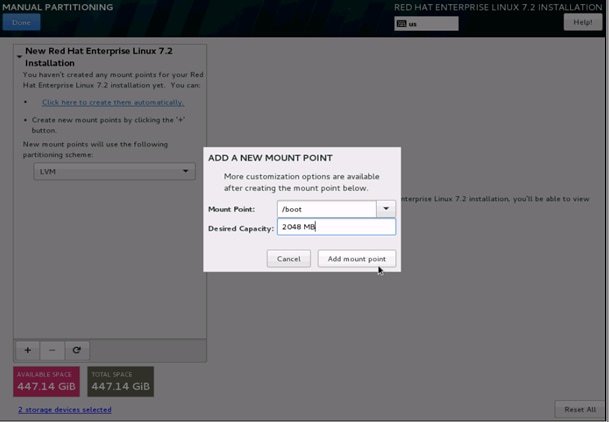
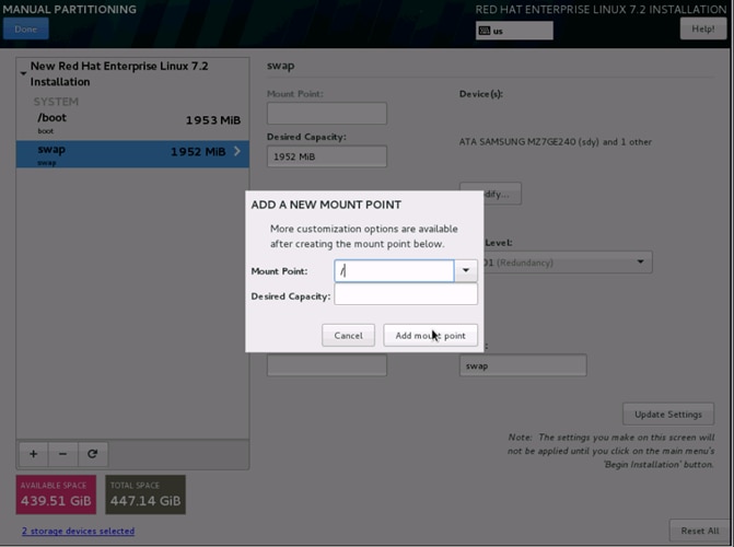
21. This opens the new window for creating the partitions. Click on the + sign to add a new partition as shown below, boot partition of size 2048 MB.
22. Click Add MountPoint to add the partition.
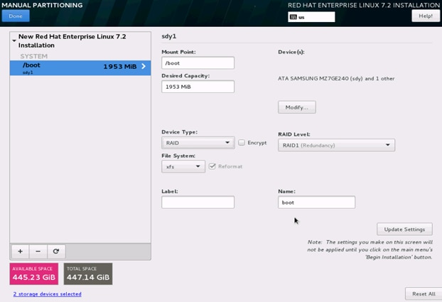
23. Change the Device type to RAID and make sure the RAID Level is RAID1 (Redundancy) and click on Update Settings to save the changes.
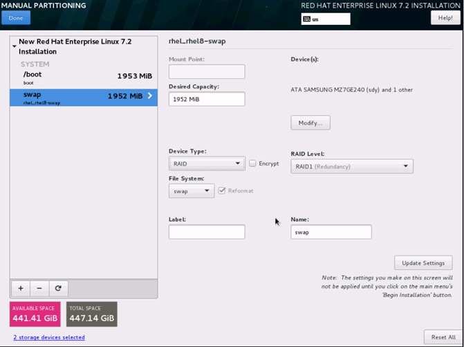
24. Click on the + sign to create the swap partition of size 2048 MB as shown below.
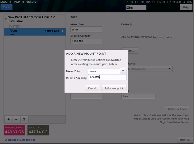
25. Change the Device type to RAID and RAID level to RAID1 (Redundancy) and click on Update Settings.
26. Click + to add the / partition. The size can be left empty so it uses the remaining capacity and click Add Mountpoint.
27. Change the Device type to RAID and RAID level to RAID1 (Redundancy).Click Update Settings.
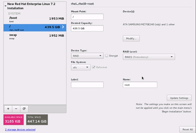
28. Click Done to go back to the main screen and continue the Installation.
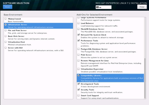
29. Click on Software Selection.

30. Select Infrastructure Server and select the Add-Ons as noted below. Click Done.
31. Click on Network and Hostname and configure Hostname and Networking for the Host.
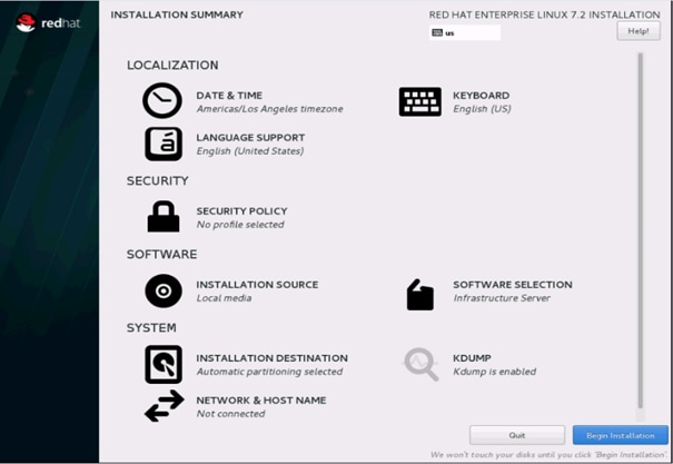
32. Type in the hostname as shown below.
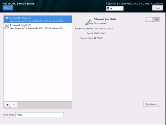
33. Click on Configure to open the Network Connectivity window. Click on IPV4Settings.
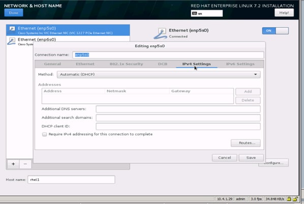
34. Change the Method to Manual and click Add to enter the IP Address, Netmask and Gateway details.
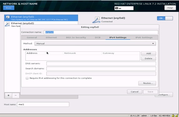
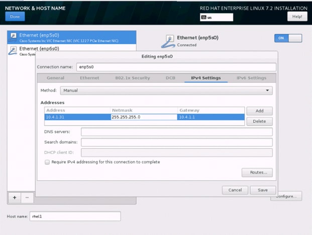
35. Click Save, update the hostname and turn Ethernet ON. Click Done to return to the main menu.
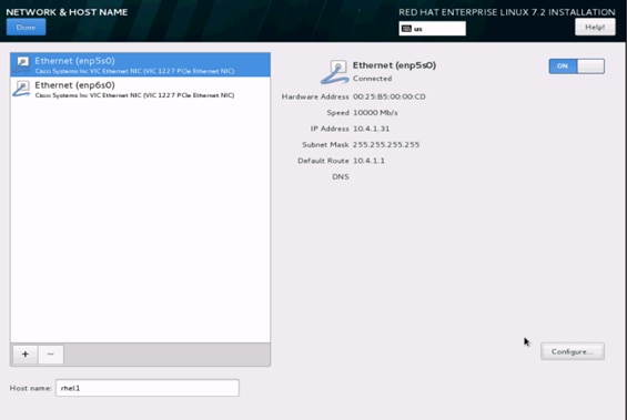
36. Click Begin Installation in the main menu.
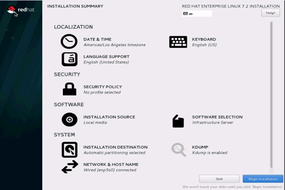
37. Select Root Password in the User Settings.
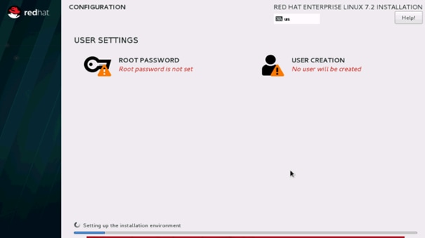
38. Enter the Root Password and click done.
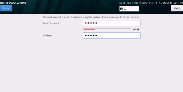
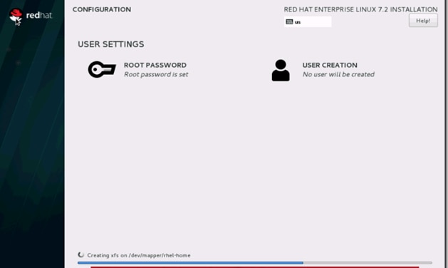
39. Once the installation is complete reboot the system.
40. Repeat steps 1 to 26 to install Red Hat Enterprise Linux 7.2 on Servers 2 through 64.
![]() Note: The OS installation and configuration of the nodes that is mentioned above can be automated through PXE boot or third party tools.
Note: The OS installation and configuration of the nodes that is mentioned above can be automated through PXE boot or third party tools.
The hostnames and their corresponding IP addresses are shown in Table 7 .
Table 7 Hostnames and IP Addresses
| Hostname |
eth0 |
| rhel1 |
10.4.1.31 |
| rhel2 |
10.4.1.32 |
| rhel3 |
10.4.1.33 |
| rhel4 |
10.4.1.34 |
| rhel1 |
10.4.1.35 |
| rhel6 |
10.4.1.36 |
| rhel7 |
10.4.1.37 |
| rhel8 |
10.4.1.38 |
| rhel9 |
10.4.1.39 |
| rhel10 |
10.4.1.40 |
| rhel11 |
10.4.1.41 |
| rhel12 |
10.4.1.42 |
| rhel13 |
10.4.1.43 |
| rhel14 |
10.4.1.44 |
| rhel15 |
10.4.1.45 |
| rhel16 |
10.4.1.46 |
| … |
… |
| rhel64 |
10.4.1.94 |
![]() Note: Cloudera does not recommend multi-homing configurations, so please assign only one network to each node.
Note: Cloudera does not recommend multi-homing configurations, so please assign only one network to each node.
Post OS Install Configuration
Choose one of the nodes of the cluster or a separate node as the Admin Node for management such as CDH installation, cluster parallel shell, creating a local Red Hat repo and others. In this document, we use rhel1 for this purpose.
Setting Up Password-less Login
To manage all of the clusters nodes from the admin node password-less login needs to be setup. It assists in automating common tasks with clustershell (clush, a cluster wide parallel shell), and shell-scripts without having to use passwords.
Once Red Hat Linux is installed across all the nodes in the cluster, follow the steps below in order to enable password-less login across all the nodes.
1. Login to the Admin Node (rhel1).
#ssh 10.4.1.31
2. Run the ssh-keygen command to create both public and private keys on the admin node.
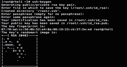
3. Then run the following command from the admin node to copy the public key id_rsa.pub to all the nodes of the cluster. ssh-copy-id appends the keys to the remote-host’s .ssh/authorized_keys.
#for IP in {31..94}; do echo -n "$IP -> "; ssh-copy-id -i ~/.ssh/id_rsa.pub 10.4.1.$IP; done
4. Enter yes for Are you sure you want to continue connecting (yes/no)?
5. Enter the password of the remote host.
Configuring /etc/hosts
Setup /etc/hosts on the Admin node; this is a pre-configuration to setup DNS as shown in the next section.
To create the host file on the admin node, complete the following steps:
1. Populate the host file with IP addresses and corresponding hostnames on the Admin node (rhel1) and other nodes as follows:
2. On Admin Node (rhel1)
#vi /etc/hosts
127.0.0.1 localhost localhost.localdomain localhost4 \ localhost4.localdomain4
::1 localhost localhost.localdomain localhost6 \ localhost6.localdomain6
10.4.1.31 rhel1
10.4.1.32 rhel2
10.4.1.33 rhel3
10.4.1.34 rhel4
10.4.1.35 rhel5
10.4.1.36 rhel6
10.4.1.37 rhel7
10.4.1.38 rhel8
10.4.1.39 rhel9
10.4.1.40 rhel10
10.4.1.41 rhel11
10.4.1.42 rhel12
10.4.1.43 rhel13
10.4.1.44 rhel14
10.4.1.45 rhel15
10.4.1.46 rhel16
...
10.4.1.94 rhel64
Creating a Red Hat Enterprise Linux (RHEL) 7.2 Local Repo
To create a repository using RHEL DVD or ISO on the admin node (in this deployment rhel1 is used for this purpose), create a directory with all the required RPMs, run the createrepo command and then publish the resulting repository.
1. Log on to rhel1. Create a directory that would contain the repository.
2. #mkdir -p /var/www/html/rhelrepo
3. Copy the contents of the Red Hat DVD to /var/www/html/rhelrepo
4. Alternatively, if you have access to a Red Hat ISO Image, Copy the ISO file to rhel1.
5. And login back to rhel1 and create the mount directory.
#scp rhel-server-7.2-x86_64-dvd.iso rhel1:/root/
#mkdir -p /mnt/rheliso
#mount -t iso9660 -o loop /root/rhel-server-7.2-x86_64-dvd.iso /mnt/rheliso/
6. Copy the contents of the ISO to the /var/www/html/rhelrepo directory.
#cp -r /mnt/rheliso/* /var/www/html/rhelrepo
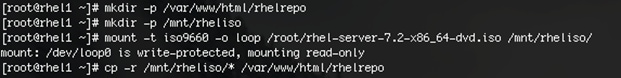
7. Now on rhel1 create a .repo file to enable the use of the yum command.
#vi /var/www/html/rhelrepo/rheliso.repo
[rhel7.2]
name=Red Hat Enterprise Linux 7.2
baseurl=http://10.4.1.31/rhelrepo
gpgcheck=0
enabled=1
8. Now copy rheliso.repo file from /var/www/html/rhelrepo to /etc/yum.repos.d on rhel1.
#cp /var/www/html/rhelrepo/rheliso.repo /etc/yum.repos.d/
![]() Note: Based on this repo file yum requires httpd to be running on rhel1 for other nodes to access the repository.
Note: Based on this repo file yum requires httpd to be running on rhel1 for other nodes to access the repository.
9. To make use of repository files on rhel1 without httpd, edit the baseurl of repo file /etc/yum.repos.d/rheliso.repo to point repository location in the file system.
![]() Note: This step is needed to install software on Admin Node (rhel1) using the repo (such as httpd, create-repo, etc.)
Note: This step is needed to install software on Admin Node (rhel1) using the repo (such as httpd, create-repo, etc.)
#vi /etc/yum.repos.d/rheliso.repo
[rhel7.2]
name=Red Hat Enterprise Linux 7.2
baseurl=file:///var/www/html/rhelrepo
gpgcheck=0
enabled=1
Creating the Red Hat Repository Database.
10. Install the createrepo package on admin node (rhel1). Use it to regenerate the repository database(s) for the local copy of the RHEL DVD contents.
#yum -y install createrepo
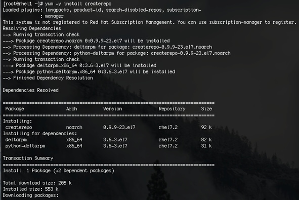
11. Run createrepo on the RHEL repository to create the repo database on admin node
#cd /var/www/html/rhelrepo
#createrepo .
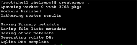
Setting up ClusterShell
ClusterShell (or clush) is the cluster-wide shell that runs commands on several hosts in parallel.
1. From the system connected to the Internet download Cluster shell (clush) and install it on rhel1. Cluster shell is available from EPEL (Extra Packages for Enterprise Linux) repository.
#wget http://rpm.pbone.net/index.php3/stat/4/idpl/31529309/dir/redhat_el_7/com/clustershell-1.7-1.el7.noarch.rpm.html
#scp clustershell-1.7-1.el7.noarch.rpm rhel1:/root/
2. Login to rhel1 and install cluster shell.
3. #yum –y install clustershell-1.71.el7.noarch.rpm
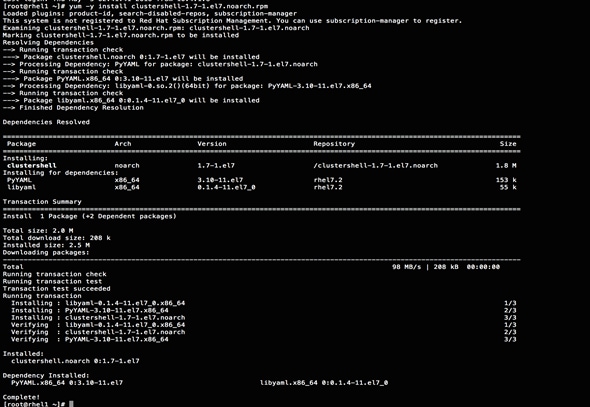
4. Edit /etc/clustershell/groups.d/local.cfg file to include hostnames for all the nodes of the cluster. This set of hosts is taken when running clush with the ‘-a’ option.
5. For 64 node cluster as in our CVD, set groups file as follows,
#vi /etc/clustershell/groups.d/local.cfg
![]()
all: rhel[1-64]
![]() Note: For more information and documentation on ClusterShell, visit https://github.com/cea-hpc/clustershell/wiki/UserAndProgrammingGuide.
Note: For more information and documentation on ClusterShell, visit https://github.com/cea-hpc/clustershell/wiki/UserAndProgrammingGuide.
![]() Note: clustershell will not work if not ssh to the machine earlier (as it requires to be in known_hosts file), for instance, as in the case below for rhel<host>.
Note: clustershell will not work if not ssh to the machine earlier (as it requires to be in known_hosts file), for instance, as in the case below for rhel<host>.
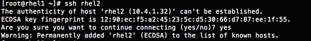
Installing httpd
Setting up RHEL repo on the admin node requires httpd. To set up RHEL repository on the admin node, complete the following steps:
1. Install httpd on the admin node to host repositories.
The Red Hat repository is hosted using HTTP on the admin node, this machine is accessible by all the hosts in the cluster.
#yum –y install httpd
2. Add ServerName and make the necessary changes to the server configuration file.
#vi /etc/httpd/conf/httpd.conf
ServerName 10.4.1.31:80

3. Start httpd
#service httpd start
#chkconfig httpd on
Set Up all Nodes to use the RHEL Repository
![]() Note: Based on this repo file yum requires httpd to be running on rhel1 for other nodes to access the repository.
Note: Based on this repo file yum requires httpd to be running on rhel1 for other nodes to access the repository.
1. Copy the rheliso.repo to all the nodes of the cluster.
#clush –w rhel[2-64] -c /var/www/html/rhelrepo/rheliso.repo --dest=/etc/yum.repos.d/
![]()
2. Also copy the /etc/hosts file to all nodes.
#clush –w rhel[2-64] –c /etc/hosts –-dest=/etc/hosts
3. Purge the yum caches after this
#clush -a -B yum clean all
#clush –a –B yum repolist
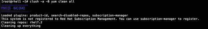
![]() Note: While suggested configuration is to disable SELinux as shown below, if for any reason SELinux needs to be enabled on the cluster, then ensure to run the following to make sure that the httpd is able to read the Yum repofiles
Note: While suggested configuration is to disable SELinux as shown below, if for any reason SELinux needs to be enabled on the cluster, then ensure to run the following to make sure that the httpd is able to read the Yum repofiles
#chcon -R -t httpd_sys_content_t /var/www/html/
Configuring DNS
This section details setting up DNS using dnsmasq as an example based on the /etc/hosts configuration setup in the earlier section.
To create the host file across all the nodes in the cluster, complete the following steps:
1. Disable Network manager on all nodes
#clush -a -b service NetworkManager stop
#clush -a -b chkconfig NetworkManager off
2. Update /etc/resolv.conf file to point to Admin Node
#vi /etc/resolv.conf
nameserver 10.4.1.31
![]() Note: This step is needed if setting up dnsmasq on Admin node. Otherwise this file should be updated with the correct nameserver.
Note: This step is needed if setting up dnsmasq on Admin node. Otherwise this file should be updated with the correct nameserver.
![]() Note: Alternatively #systemctl start NetworkManager.service can be used to start the service. #systemctl stop NetworkManager.service can be used to stop the service. Use #systemctl disable NetworkManager.service to stop a service from being automatically started at boot time.
Note: Alternatively #systemctl start NetworkManager.service can be used to start the service. #systemctl stop NetworkManager.service can be used to stop the service. Use #systemctl disable NetworkManager.service to stop a service from being automatically started at boot time.
3. Install and Start dnsmasq on Admin node
#service dnsmasq start
#chkconfig dnsmasq on
4. Deploy /etc/resolv.conf from the admin node (rhel1) to all the nodes via the following clush command:
#clush -a -B -c /etc/resolv.conf
![]() Note: A clush copy without –dest copies to the same directory location as the source-file directory
Note: A clush copy without –dest copies to the same directory location as the source-file directory
5. Ensure DNS is working fine by running the following command on Admin node and any data-node
[root@rhel2 ~]# nslookup rhel1
Server: 10.4.1.31
Address: 10.4.1.31#53
Name: rhel1
Address: 10.4.1.31 ç
![]() Note: yum install –y bind-utils will need to be run for nslookup to utility to run.
Note: yum install –y bind-utils will need to be run for nslookup to utility to run.
Upgrading the Cisco Network driver for VIC1227
The latest Cisco Network driver is required for performance and updates. The latest drivers can be downloaded from the link below:
https://software.cisco.com/download/release.html?mdfid=286281356&reltype=latest&relind=AVAILABLE&dwnld=true&softwareid=283853158&rellifecycle=&atcFlag=N&release=2.0%289b%29&dwldImageGuid=84C2FF3BB579A1BF32F7227C59F6DF886CEDBE99&flowid=71443
1. In the ISO image, the required driver kmod-enic-2.3.0.20-rhel7u2.el7.x86_64.rpm can be located at \Linux\Network\Cisco\VIC\RHEL\RHEL7.2.
2. From a node connected to the Internet, download, extract and transfer kmod-enic-2.3.0.20-rhel7u2.el7.x86_64.rpm to rhel1 (admin node).
3. Install the rpm on all nodes of the cluster using the following clush commands. For this example the rpm is assumed to be in present working directory of rhel1.
4. [root@rhel1 ~]# clush -a -b -c kmod-enic-2.3.0.20-rhel7u2.el7.x86_64.rpm
5. [root@rhel1 ~]# clush -a -b "rpm –ivh kmod-enic-2.3.0.20-rhel7u2.el7.x86_64.rpm"
6. Ensure that the above installed version of kmod-enic driver is being used on all nodes by running the command "modinfo enic" on all nodes
[root@rhel1 ~]# clush -a -B "modinfo enic | head -5"
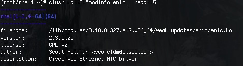
7. Also it is recommended to download the kmod-megaraid driver for higher performance , the RPM can be found in the same package at \Linux\Storage\LSI\Cisco_Storage_12G_SAS_RAID_controller\RHEL\RHEL7.2
Installing xfsprogs
From the admin node rhel1 run the command below to Install xfsprogs on all the nodes for xfs filesystem.
#clush -a -B yum -y install xfsprogs
![]()
NTP Configuration
The Network Time Protocol (NTP) is used to synchronize the time of all the nodes within the cluster. The Network Time Protocol daemon (ntpd) sets and maintains the system time of day in synchronism with the timeserver located in the admin node (rhel1). Configuring NTP is critical for any Hadoop Cluster. If server clocks in the cluster drift out of sync, serious problems will occur with HBase and other services.
#clush –a –b "yum –y install ntp"
|
|
|
1. Configure /etc/ntp.conf on the admin node only with the following contents:
#vi /etc/ntp.conf
driftfile /var/lib/ntp/drift
restrict 127.0.0.1
restrict -6 ::1
server 127.127.1.0
fudge 127.127.1.0 stratum 10
includefile /etc/ntp/crypto/pw
keys /etc/ntp/keys
2. Create /root/ntp.conf on the admin node and copy it to all nodes
#vi /root/ntp.conf
server 10.4.1.31
driftfile /var/lib/ntp/drift
restrict 127.0.0.1
restrict -6 ::1
includefile /etc/ntp/crypto/pw
keys /etc/ntp/keys
3. Copy ntp.conf file from the admin node to /etc of all the nodes by executing the following command in the admin node (rhel1)
#for SERVER in {32..94}; do scp /root/ntp.conf 10.4.1.$SERVER:/etc/ntp.conf; done
![]()
![]() Note: Instead of the above for loop, this could be run as a clush command with "–w"option.
Note: Instead of the above for loop, this could be run as a clush command with "–w"option.
#clush -w rhel[2-94] –b –c /root/ntp.conf --dest=/etc
4. Run the following to syncronize the time and restart NTP daemon on all nodes.
#clush -a -b "service ntpd stop"
#clush -a -b "ntpdate rhel1"
#clush -a -b "service ntpd start"
5. Ensure restart of NTP daemon across reboots
#clush –a –b "systemctl enable ntpd"
Alternatively, the new Chrony service can be installed, that is quicker to synchronize clocks in mobile and virtual systems.
6. Install the Chrony service:
# yum install -y chrony
7. Activate the Chrony service at boot:
8. # systemctl enable chronyd
9. Start the Chrony service:
# systemctl start chronyd
The Chrony configuration is in the /etc/chrony.conf file, configured similar to /etc/ntp.conf.
Enabling Syslog
Syslog must be enabled on each node to preserve logs regarding killed processes or failed jobs. Modern versions such as syslog-ng and rsyslog are possible, making it more difficult to be sure that a syslog daemon is present. One of the following commands should suffice to confirm that the service is properly configured:
#clush -B -a rsyslogd –v
#clush -B -a service rsyslog status
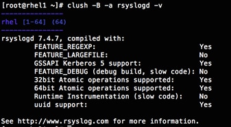
Setting ulimit
On each node, ulimit -n specifies the number of inodes that can be opened simultaneously. With the default value of 1024, the system appears to be out of disk space and shows no inodes available. This value should be set to 64000 on every node.
Higher values are unlikely to result in an appreciable performance gain.
1. For setting the ulimit on Redhat, edit /etc/security/limits.conf on admin node rhel1 and add the following lines:
root soft nofile 64000
root hard nofile 64000

2. Copy the /etc/security/limits.conf file from admin node (rhel1) to all the nodes using the following command.
#clush -a -b -c /etc/security/limits.conf --dest=/etc/security/
![]()
3. Check that the /etc/pam.d/su file contains the following settings:
#%PAM-1.0
auth sufficient pam_rootOK.so
# Uncomment the following line to implicitly trust users in the "wheel" group.
#auth sufficient pam_wheel.so trust use_uid
# Uncomment the following line to require a user to be in the "wheel" group.
#auth required pam_wheel.so use_uid
auth include system-auth
account sufficient pam_succeed_if.so uid = 0 use_uid quiet
account include system-auth
password include system-auth
session include system-auth
session optional pam_xauth.so
![]() Note: The ulimit values are applied on a new shell, running the command on a node on an earlier instance of a shell will show old values.
Note: The ulimit values are applied on a new shell, running the command on a node on an earlier instance of a shell will show old values.
Disabling SELinux
SELinux must be disabled during the install procedure and cluster setup. SELinux can be enabled after installation and while the cluster is running.
SELinux can be disabled by editing /etc/selinux/config and changing the SELINUX line to SELINUX=disabled. The following command will disable SELINUX on all nodes.
#clush -a -b "sed –i 's/SELINUX=enforcing/SELINUX=disabled/g' /etc/selinux/config"
![]()
#clush –a –b "setenforce 0"
![]() Note: The above command may fail if SELinux is already disabled.
Note: The above command may fail if SELinux is already disabled.
Reboot the machine, if needed for SELinux to be disabled incase it does not take effect. It can checked using
#clush –a –b sestatus
Set TCP Retries
Adjusting the tcp_retries parameter for the system network enables faster detection of failed nodes. Given the advanced networking features of UCS, this is a safe and recommended change (failures observed at the operating system layer are most likely serious rather than transitory). On each node, set the number of TCP retries to 5 can help detect unreachable nodes with less latency.
1. Edit the file /etc/sysctl.conf and on admin node rhel1 and add the following lines:
net.ipv4.tcp_retries2=5
2. Copy the /etc/sysctl.conf file from admin node (rhel1) to all the nodes using the following command:
#clush -a -b -c /etc/sysctl.conf --dest=/etc/
3. Load the settings from default sysctl file /etc/sysctl.conf by running.
#clush -B -a sysctl -p
Disabling the Linux Firewall
The default Linux firewall settings are far too restrictive for any Hadoop deployment. Since the UCS Big Data deployment will be in its own isolated network there is no need for that additional firewall.
#clush -a -b " firewall-cmd --zone=public --add-port=80/tcp --permanent"
#clush -a -b "firewall-cmd --reload"
#clush –a –b “systemctl disable firewalld”
Disable Swapping
1. In order to reduce Swapping, run the following on all nodes. Variable vm.swappiness defines how often swap should be used, 60 is default.
#clush -a -b " echo 'vm.swappiness=1' >> /etc/sysctl.conf"
2. Load the settings from default sysctl file /etc/sysctl.conf.
#clush –a –b "sysctl –p"
Disable Transparent Huge Pages
Disabling Transparent Huge Pages (THP) reduces elevated CPU usage caused by THP.
#clush -a -b "echo never > /sys/kernel/mm/transparent_hugepage/enabled”
#clush -a -b "echo never > /sys/kernel/mm/transparent_hugepage/defrag"
1. The above commands must be run for every reboot, so copy this command to /etc/rc.local so they are executed automatically for every reboot.
2. On the Admin node, run the following commands
#rm –f /root/thp_disable
#echo "echo never > /sys/kernel/mm/transparent_hugepage/enabled" >>
/root/thp_disable
#echo "echo never > /sys/kernel/mm/transparent_hugepage/defrag " >>
/root/thp_disable
3. Copy file to each node
#clush –a –b –c /root/thp_disable
4. Append the content of file thp_disable to /etc/rc.local
#clush -a -b “cat /root/thp_disable >> /etc/rc.local”
Disable IPv6 Defaults
1. Disable IPv6 as the addresses used are IPv4.
#clush -a -b "echo 'net.ipv6.conf.all.disable_ipv6 = 1' >> /etc/sysctl.conf"
#clush -a -b "echo 'net.ipv6.conf.default.disable_ipv6 = 1' >> /etc/sysctl.conf"
#clush -a -b "echo 'net.ipv6.conf.lo.disable_ipv6 = 1' >> /etc/sysctl.conf"
2. Load the settings from default sysctl file /etc/sysctl.conf.
#clush –a –b "sysctl –p"
Configuring Data Drives on Name Node And Other Management Nodes
This section describes steps to configure non-OS disk drives as RAID1 using StorCli command as described below. All the drives are going to be part of a single RAID1 volume. This volume can be used for Staging any client data to be loaded to HDFS. This volume won’t be used for HDFS data.
1. From the website download storcli http://www.lsi.com/downloads/Public/RAID%20Controllers/RAID%20Controllers%20Common%20Files/1.14.12_StorCLI.zip
2. Extract the zip file and copy storcli-1.14.12-1.noarch.rpm from the linux directory.
3. Download storcli and its dependencies and transfer to Admin node.
#scp storcli-1.14.12-1.noarch.rpm rhel1:/root/
4. Copy storcli rpm to all the nodes using the following commands:
#clush -a -b -c /root/storcli-1.14.12-1.noarch.rpm --dest=/root/
5. Run the below command to install storcli on all the nodes
#clush -a -b “rpm -ivh storcli-1.14.12-1.noarch.rpm”
6. Run the below command to copy storcli64 to root directory.
#cd /opt/MegaRAID/storcli/
#cp storcli64 /root/

7. Copy storcli64 to all the nodes using the following commands:
#clush -a -b -c /root/storcli64 --dest=/root/
8. Run the following script as root user on rhel1 to rhel3 to create the virtual drives for the management nodes.
#vi /root/raid1.sh
./storcli64 -cfgldadd r1[$1:1,$1:2,$1:3,$1:4,$1:5,$1:6,$1:7,$1:8,$1:9,$1:10,$1:11,$1:12,$1:13,$1:14,$1:15,$1:16,$1:17,$1:18,$1:19,$1:20,$1:21,$1:22,$1:23,$1:24] wb ra nocachedbadbbu strpsz1024 -a0
The above script requires enclosure ID as a parameter.
9. Run the following command to get enclosure id.
#./storcli64 pdlist -a0 | grep Enc | grep -v 252 | awk '{print $4}' | sort | uniq -c | awk '{print $2}'
#chmod 755 raid1.sh
10. Run MegaCli script as follows
#./raid1.sh <EnclosureID> obtained by running the command above
WB: Write back
RA: Read Ahead
NoCachedBadBBU: Do not write cache when the BBU is bad.
Strpsz1024: Strip Size of 1024K
![]() Note: The command above will not override any existing configuration. To clear and reconfigure existing configurations refer to Embedded MegaRAID Software Users Guide available at www.lsi.com.
Note: The command above will not override any existing configuration. To clear and reconfigure existing configurations refer to Embedded MegaRAID Software Users Guide available at www.lsi.com.
Cloudera recommends the following disk configuration for the master nodes.
· At least 10 physical disks in following configuration
· 2 x RAID1 OS (Root disk)
· 4 x RAID 10 (DB filesystems)
· 2 x RAID 1 HDFS NameNode metadata
· 1 x JBOD - ZooKeeper
· 1 x JBOD - Quorum JournalNode
Configuring Data Drives on Data Nodes
This section describes steps to configure non-OS disk drives as individual RAID0 volumes using StorCli command as described below. These volumes are going to be used for HDFS Data.
1. Issue the following command from the admin node to create the virtual drives with individual RAID 0 configurations on all the data nodes.
#clush –w rhel[3-64] -B ./storcli64 -cfgeachdskraid0 WB RA direct NoCachedBadBBU strpsz1024 -a0
WB: Write back
RA: Read Ahead
NoCachedBadBBU: Do not write cache when the BBU is bad.
Strpsz1024: Strip Size of 1024K
![]() Note: The command above will not override existing configurations. To clear and reconfigure existing configurations refer to Embedded MegaRAID Software Users Guide available at www.lsi.com.
Note: The command above will not override existing configurations. To clear and reconfigure existing configurations refer to Embedded MegaRAID Software Users Guide available at www.lsi.com.
Configuring the Filesystem for NameNodes and Datanodes
The following script will format and mount the available volumes on each node whether it is Namenode or Data node. OS boot partition is going to be skipped. All drives are going to be mounted based on their UUID as /data/disk1, /data/disk2, and so on.
1. On the Admin node, create a file containing the following script.
2. To create partition tables and file systems on the local disks supplied to each of the nodes, run the following script as the root user on each node.
![]() Note: The script assumes there are no partitions already existing on the data volumes. If there are partitions, delete them before running the script. This process is documented in the "Note" section at the end of the section.
Note: The script assumes there are no partitions already existing on the data volumes. If there are partitions, delete them before running the script. This process is documented in the "Note" section at the end of the section.
#vi /root/driveconf.sh
#!/bin/bash
#disks_count=`lsblk -id | grep sd | wc -l`
#if [ $disks_count -eq 24 ]; then
# echo "Found 24 disks"
#else
# echo "Found $disks_count disks. Expecting 24. Exiting.."
# exit 1
#fi
[[ "-x" == "${1}" ]] && set -x && set -v && shift 1
count=1
for X in /sys/class/scsi_host/host?/scan
do
echo '- - -' > ${X}
done
for X in /dev/sd?
do
echo "========"
echo $X
echo "========"
if [[ -b ${X} && `/sbin/parted -s ${X} print quit|/bin/grep -c boot` -ne 0
]]
then
echo "$X bootable - skipping."
continue
else
Y=${X##*/}1
echo "Formatting and Mounting Drive => ${X}"
/sbin/mkfs.xfs -f ${X}
(( $? )) && continue
#Identify UUID
UUID=`blkid ${X} | cut -d " " -f2 | cut -d "=" -f2 | sed 's/"//g'`
/bin/mkdir -p /data/disk${count}
(( $? )) && continue
echo "UUID of ${X} = ${UUID}, mounting ${X} using UUID on /data/disk${count}"
/bin/mount -t xfs -o inode64,noatime,nobarrier -U ${UUID} /data/disk${count}
(( $? )) && continue
echo "UUID=${UUID} /data/disk${count} xfs inode64,noatime,nobarrier 0 0" >> /etc/fstab
((count++))
fi
done
3. Run the following command to copy driveconf.sh to all the nodes:
#chmod 755 /root/driveconf.sh
#clush –a -B –c /root/driveconf.sh
4. Run the following command from the admin node to run the script across all data nodes
#clush –a –B /root/driveconf.sh
5. Run the following from the admin node to list the partitions and mount points
#clush –a -B df –h
#clush –a -B mount
#clush –a -B cat /etc/fstab
![]() Note: In-case there is a need to delete any partitions, it can be done so using the following.
Note: In-case there is a need to delete any partitions, it can be done so using the following.
6. Run the mount command (‘mount’) to identify which drive is mounted to which device /dev/sd<?>
7. umount the drive for which partition is to be deleted and run fdisk to delete as shown below.
![]() Note: Care should be taken not to delete the OS partition as this will wipe out the OS.
Note: Care should be taken not to delete the OS partition as this will wipe out the OS.
#mount
#umount /data/disk1 ç (disk1 shown as example)
#(echo d; echo w;) | sudo fdisk /dev/sd<?>
Cluster Verification
This section describes the steps to create the script cluster_verification.sh that helps to verify the CPU, memory, NIC, and storage adapter settings across the cluster on all nodes. This script also checks additional prerequisites such as NTP status, SELinux status, ulimit settings, JAVA_HOME settings and JDK version, IP address and hostname resolution, Linux version and firewall settings.
1. Create the script cluster_verification.sh as shown, on the Admin node (rhel1).
#vi cluster_verification.sh
#!/bin/bash
shopt -s expand_aliases,
# Setting Color codes
green='\e[0;32m'
red='\e[0;31m'
NC='\e[0m' # No Color
echo -e "${green} === Cisco UCS Integrated Infrastructure for Big Data and Analytics \ Cluster Verification === ${NC}"
echo ""
echo ""
echo -e "${green} ==== System Information ==== ${NC}"
echo ""
echo ""
echo -e "${green}System ${NC}"
clush -a -B " `which dmidecode` |grep -A2 '^System Information'"
echo ""
echo ""
echo -e "${green}BIOS ${NC}"
clush -a -B " `which dmidecode` | grep -A3 '^BIOS I'"
echo ""
echo ""
echo -e "${green}Memory ${NC}"
clush -a -B "cat /proc/meminfo | grep -i ^memt | uniq"
echo ""
echo ""
echo -e "${green}Number of Dimms ${NC}"
clush -a -B "echo -n 'DIMM slots: '; `which dmidecode` |grep -c \ '^[[:space:]]*Locator:'"
clush -a -B "echo -n 'DIMM count is: '; `which dmidecode` | grep \ "Size"| grep -c "MB""
clush -a -B " `which dmidecode` | awk '/Memory Device$/,/^$/ {print}' |\ grep -e '^Mem' -e Size: -e Speed: -e Part | sort -u | grep -v -e 'NO \ DIMM' -e 'No Module Installed' -e Unknown"
echo ""
echo ""
# probe for cpu info #
echo -e "${green}CPU ${NC}"
clush -a -B "grep '^model name' /proc/cpuinfo | sort -u"
echo ""
clush -a -B "`which lscpu` | grep -v -e op-mode -e ^Vendor -e family -e\ Model: -e Stepping: -e BogoMIPS -e Virtual -e ^Byte -e '^NUMA node(s)'"
echo ""
echo ""
# probe for nic info #
echo -e "${green}NIC ${NC}"
clush -a -B "`which ifconfig` | egrep '(^e|^p)' | awk '{print \$1}' | \ xargs -l `which ethtool` | grep -e ^Settings -e Speed"
echo ""
clush -a -B "`which lspci` | grep -i ether"
echo ""
echo ""
# probe for disk info #
echo -e "${green}Storage ${NC}"
clush -a -B "echo 'Storage Controller: '; `which lspci` | grep -i -e \ raid -e storage -e lsi"
echo ""
clush -a -B "dmesg | grep -i raid | grep -i scsi"
echo ""
clush -a -B "lsblk -id | awk '{print \$1,\$4}'|sort | nl"
echo ""
echo ""
echo -e "${green} ================ Software ======================= ${NC}"
echo ""
echo ""
echo -e "${green}Linux Release ${NC}"
clush -a -B "cat /etc/*release | uniq"
echo ""
echo ""
echo -e "${green}Linux Version ${NC}"
clush -a -B "uname -srvm | fmt"
echo ""
echo ""
echo -e "${green}Date ${NC}"
clush -a -B date
echo ""
echo ""
echo -e "${green}NTP Status ${NC}"
clush -a -B "ntpstat 2>&1 | head -1"
echo ""
echo ""
echo -e "${green}SELINUX ${NC}"
clush -a -B "echo -n 'SElinux status: '; grep ^SELINUX= \ /etc/selinux/config 2>&1"
echo ""
echo ""
clush -a -B "echo -n 'CPUspeed Service: '; `which service` cpuspeed \ status 2>&1"
clush -a -B "echo -n 'CPUspeed Service: '; `which chkconfig` --list \ cpuspeed 2>&1"
echo ""
echo ""
echo -e "${green}Java Version${NC}"
clush -a -B 'java -version 2>&1; echo JAVA_HOME is ${JAVA_HOME:-Not \ Defined!}'
echo ""
echo ""
echo -e "${green}Hostname LoOKup${NC}"
clush -a -B " ip addr show"
echo ""
echo ""
echo -e "${green}Open File Limit${NC}"
clush -a -B 'echo -n "Open file limit(should be >32K): "; ulimit -n'
2. Change permissions to executable.
chmod 755 cluster_verification.sh
3. Run the Cluster Verification tool from the admin node. This can be run before starting Hadoop to identify any discrepancies in Post OS Configuration between the servers or during troubleshooting of any cluster / Hadoop issues.
#./cluster_verification.sh
Installing Cloudera
Cloudera’s Distribution including Apache Hadoop (CDH) is an enterprise grade, hardened Hadoop distribution. CDH offers Apache Hadoop and several related projects into a single tested and certified product. It offers the latest innovations from the open source community with the testing and quality expected from enterprise quality software.
Pre-Requisites for CDH Installation
This section details the prerequisites for CDH installation such as setting up CDH Repo.
Cloudera Manager Repository
1. From a host connected to the Internet, download the Cloudera’s repositories as shown below and transfer it to the admin node.
#mkdir -p /tmp/clouderarepo/
2. Download Cloudera Manager Repository.
#cd /tmp/clouderarepo/
#wget http:/ /archive.cloudera.com/cm5/redhat/7/x86_64/cm/cloudera-manager.repo
#reposync --config=./cloudera-manager.repo --repoid=cloudera-manager
This downloads the Cloudera Manager RPMs needed for the Cloudera repository.
3. Run the following command to move the RPMs
4. Copy the repository directory to the admin node (rhel1)
#scp -r /tmp/clouderarepo/ rhel1:/var/www/html/
5. On admin node (rhel1) run create repo command.
#cd /var/www/html/clouderarepo/
#createrepo --baseurl http://10.4.1.31/clouderarepo/cloudera-manager/
/var/www/html/clouderarepo/cloudera-manager

![]() Note: Visit http://10.4.1.31/clouderarepo/ to verify the files.
Note: Visit http://10.4.1.31/clouderarepo/ to verify the files.
6. Create the Cloudera Manager repo file with following contents:
#vi /var/www/html/clouderarepo/cloudera-manager/cloudera-manager.repo
baseurl=http://10.4.1.31/clouderarepo/cloudera-manager/
enabled=1
7. Copy the file cloudera-manager.repo into /etc/yum.repos.d/ on the admin node to enable it to find the packages that are locally hosted.
#cp /var/www/html/clouderarepo/cloudera-manager/cloudera-manager.repo /etc/yum.repos.d/
8. From the admin node copy the repo files to /etc/yum.repos.d/ of all the nodes of the cluster.
9. #clush –a –B -c /etc/yum.repos.d/cloudera-manager.repo
Setting up the Local Parcels for CDH 5.7.0
1. From a host connected the internet, download the appropriate CDH 5.7.0 parcels that are meant for RHEL7.2 from the URL: http://archive.cloudera.com/cdh5/parcels/ and place them in the directory "/var/www/html/CDH5.7parcels" of the Admin node.
The following list shows the relevant files for RHEL7.2, as shown in the figure below:
· CDH-5.7.0-1.cdh5.7.0.p0.45-el7.parcel
· CDH-5.7.0-1.cdh5.7.0.p0.45-el7.parcel.sha1 and
· manifest.json.
![]()
![]()
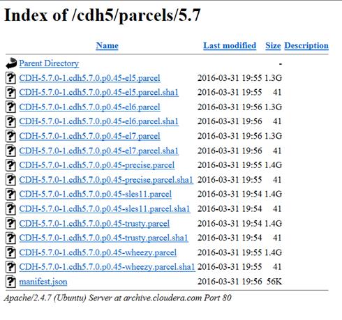
Downloading Parcels
1. From a host connected to the Internet, download the Cloudera’s parcels as shown below and transfer it to the admin node.
#mkdir -p /tmp/clouderarepo/CDH5.7parcel
2. Download parcels:
#cd /tmp/clouderarepo/CDH5.7parcels
#wget http://archive.cloudera.com/cdh5/parcels/5.7/CDH-5.7.0-1.cdh5.7.0.p0.45-el7.parcel
#wget http://archive.cloudera.com/cdh5/parcels/5.7/CDH-5.7.0-1.cdh5.7.0.p0.45-el7.parcel.sha1
#wget http://archive.cloudera.com/cdh5/parcels/5.7/manifest.json
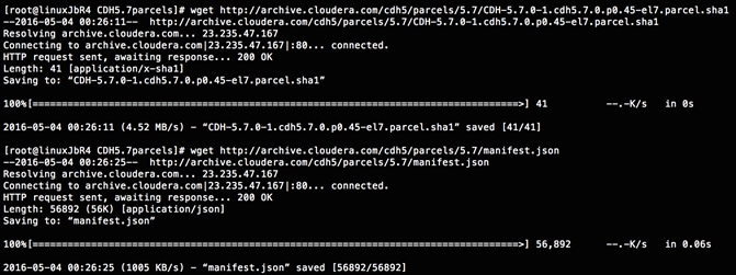
3. Now edit the /tmp/clouderarepo/CDH5.7parcels/manifest.json file and remove the scripts that are not meant for RHEL7.2. Below is that script which can be copy and pasted.
![]() Note: Please make sure the script starts and end with initial additional braces.
Note: Please make sure the script starts and end with initial additional braces.
{ {
"lastUpdated": 14594540550000,
"parcels": [
{
"parcelName": "CDH-5.7.0-1.cdh5.7.0.p0.45-el7.parcel",
"components": [
{
"pkg_version": "0.7.0+cdh5.7.0+0",
"pkg_release": "1.cdh5.7.0.p0.78",
"name": "bigtop-tomcat",
"version": "6.0.44-cdh5.7.0"
},
{
"pkg_version": "0.11.0+cdh5.7.0+93",
"pkg_release": "1.cdh5.7.0.p0.78",
"name": "crunch",
"version": "0.11.0-cdh5.7.0"
},
{
"pkg_version": "1.6.0+cdh5.7.0+37",
"pkg_release": "1.cdh5.7.0.p0.79",
"name": "flume-ng",
"version": "1.6.0-cdh5.7.0"
},
{
"pkg_version": "2.6.0+cdh5.7.0+1280",
"pkg_release": "1.cdh5.7.0.p0.92",
"name": "hadoop-0.20-mapreduce",
"version": "2.6.0-cdh5.7.0"
},
{
"pkg_version": "2.6.0+cdh5.7.0+1280",
"pkg_release": "1.cdh5.7.0.p0.92",
"name": "hadoop",
"version": "2.6.0-cdh5.7.0"
},
{
"pkg_version": "2.6.0+cdh5.7.0+1280",
"pkg_release": "1.cdh5.7.0.p0.92",
"name": "hadoop-hdfs",
"version": "2.6.0-cdh5.7.0"
},
{
"pkg_version": "2.6.0+cdh5.7.0+1280",
"pkg_release": "1.cdh5.7.0.p0.92",
"name": "hadoop-httpfs",
"version": "2.6.0-cdh5.7.0"
},
{
"pkg_version": "2.6.0+cdh5.7.0+1280",
"pkg_release": "1.cdh5.7.0.p0.92",
"name": "hadoop-kms",
"version": "2.6.0-cdh5.7.0"
},
{
"pkg_version": "2.6.0+cdh5.7.0+1280",
"pkg_release": "1.cdh5.7.0.p0.92",
"name": "hadoop-mapreduce",
"version": "2.6.0-cdh5.7.0"
},
{
"pkg_version": "2.6.0+cdh5.7.0+1280",
"pkg_release": "1.cdh5.7.0.p0.92",
"name": "hadoop-yarn",
"version": "2.6.0-cdh5.7.0"
},
{
"pkg_version": "1.2.0+cdh5.7.0+129",
"pkg_release": "1.cdh5.7.0.p0.88",
"name": "hbase",
"version": "1.2.0-cdh5.7.0"
},
{
"pkg_version": "1.5+cdh5.7.0+64",
"pkg_release": "1.cdh5.7.0.p0.78",
"name": "hbase-solr",
"version": "1.5-cdh5.7.0"
},
{
"pkg_version": "1.1.0+cdh5.7.0+522",
"pkg_release": "1.cdh5.7.0.p0.88",
"name": "hive",
"version": "1.1.0-cdh5.7.0"
},
{
"pkg_version": "1.1.0+cdh5.7.0+522",
"pkg_release": "1.cdh5.7.0.p0.88",
"name": "hive-hcatalog",
"version": "1.1.0-cdh5.7.0"
},
{
"pkg_version": "3.9.0+cdh5.7.0+1759",
"pkg_release": "1.cdh5.7.0.p0.86",
"name": "hue",
"version": "3.9.0-cdh5.7.0"
},
{
"pkg_version": "2.5.0+cdh5.7.0+0",
"pkg_release": "1.cdh5.7.0.p0.147",
"name": "impala",
"version": "2.5.0-cdh5.7.0"
},
{
"pkg_version": "1.0.0+cdh5.7.0+130",
"pkg_release": "1.cdh5.7.0.p0.77",
"name": "kite",
"version": "1.0.0-cdh5.7.0"
},
{
"pkg_version": "1.0.0+cdh5.7.0+0",
"pkg_release": "1.cdh5.7.0.p0.78",
"name": "llama",
"version": "1.0.0-cdh5.7.0"
},
{
"pkg_version": "0.9+cdh5.7.0+29",
"pkg_release": "1.cdh5.7.0.p0.79",
"name": "mahout",
"version": "0.9-cdh5.7.0"
},
{
"pkg_version": "4.1.0+cdh5.7.0+267",
"pkg_release": "1.cdh5.7.0.p0.78",
"name": "oozie",
"version": "4.1.0-cdh5.7.0"
},
{
"pkg_version": "1.5.0+cdh5.7.0+176",
"pkg_release": "1.cdh5.7.0.p0.78",
"name": "parquet",
"version": "1.5.0-cdh5.7.0"
},
{
"pkg_version": "0.12.0+cdh5.7.0+84",
"pkg_release": "1.cdh5.7.0.p0.77",
"name": "pig",
"version": "0.12.0-cdh5.7.0"
},
{
"pkg_version": "1.5.1+cdh5.7.0+184",
"pkg_release": "1.cdh5.7.0.p0.86",
"name": "sentry",
"version": "1.5.1-cdh5.7.0"
},
{
"pkg_version": "4.10.3+cdh5.7.0+389",
"pkg_release": "1.cdh5.7.0.p0.85",
"name": "solr",
"version": "4.10.3-cdh5.7.0"
},
{
"pkg_version": "1.6.0+cdh5.7.0+180",
"pkg_release": "1.cdh5.7.0.p0.84",
"name": "spark",
"version": "1.6.0-cdh5.7.0"
},
{
"pkg_version": "1.99.5+cdh5.7.0+38",
"pkg_release": "1.cdh5.7.0.p0.79",
"name": "sqoop2",
"version": "1.99.5-cdh5.7.0"
},
{
"pkg_version": "1.4.6+cdh5.7.0+56",
"pkg_release": "1.cdh5.7.0.p0.78",
"name": "sqoop",
"version": "1.4.6-cdh5.7.0"
},
{
"pkg_version": "0.9.0+cdh5.7.0+19",
"pkg_release": "1.cdh5.7.0.p0.78",
"name": "whirr",
"version": "0.9.0-cdh5.7.0"
},
{
"pkg_version": "3.4.5+cdh5.7.0+94",
"pkg_release": "1.cdh5.7.0.p0.80",
"name": "zookeeper",
"version": "3.4.5-cdh5.7.0"
}
],
"replaces": "IMPALA, SOLR, SPARK",
"hash": "6414b81d5ba5147abe67df63a55747fb47edb76e"
}
]
}
4. Copy /tmp/clouderarepo/CDH5.7parcels to the admin node (rhel1)
#scp -r /tmp/clouderarepo/CDH5.7parcels/ rhel1:/var/www/html/
5. Verify that these files are accessible by visiting the URL http://10.4.1.31/CDH5.7parcels/ in admin node.
Setting Up the MariaDB Database for Cloudera Manager
· Install the MariaDB Server
· Configure and Start the MariaDB Server
· Install the MariaDB/MySQL JDBC Driver
· Create Databases for Activity Monitor, Reports Manager, Hive Metastore Server, Sentry Server, Cloudera Navigator Audit Server, and Cloudera Navigator Metadata Server
Installing the MariaDB Server
To use a MariaDB database, complete the following steps:
1. In the admin node where Cloudera Manager will be installed, use the following command to install the mariadb/mysql server.
#yum –y install mariadb-server
2. To configure and start the MySQL Server, stop the MariaDB server if it is running.
#service mariadb stop
3. Move the old InnoDB log if exists.
4. Move files /var/lib/mysql/ib_logfile0 and /var/lib/mysql/ib_logfile1 out of/var/lib/mysql/ to a backup location.
#mv /var/lib/mysql/ib_logfile0 /root/ib_logfile0.bkp
#mv /var/lib/mysql/ib_logfile1 /root/ib_logfile1.bkp
5. Determine the location of the option file, my.cnf and edit/add following lines:
#vi /etc/my.cnf
[mysqld]
transaction-isolation = READ-COMMITTED
# InnoDB settings
innodb_flush_method = O_DIRECT
max_connections = 550
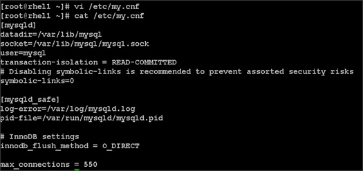
![]() Note: The max_connections need to be increased based on number of nodes and applications. Please follow the recommendations as mentioned in the Cloudera document http://www.cloudera.com/documentation/enterprise/latest/topics/install_cm_mariadb.html - install_cm_mariadb_config
Note: The max_connections need to be increased based on number of nodes and applications. Please follow the recommendations as mentioned in the Cloudera document http://www.cloudera.com/documentation/enterprise/latest/topics/install_cm_mariadb.html - install_cm_mariadb_config
6. Ensure MySQL Server starts at boot:
#systemctl enable mariadb.service
7. Start the MySQL Server:
#service mariadb start
8. Set the MySQL root password on admin node (rhel1)
#cd /usr/bin/
#mysql_secure_installation
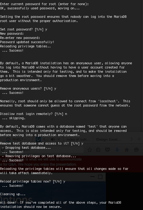
Installing the MySQL JDBC Driver
Install the JDBC driver on the Cloudera Manager Server host, as well as hosts which run the Activity Monitor, Reports Manager, Hive Metastore Server, Sentry Server, Cloudera Navigator Audit Server, and Cloudera Navigator Metadata Server roles.
1. From a host connected to the Internet, download the MySQL JDBC Driver and transfer it to the admin node. Download the MySQL JDBC driver from the URL http://www.mysql.com/downloads/connector/j/5.1.html
2. Copy mysql-connector-java-5.1.37.tar.gz to admin node(rhel1)
#scp mysql-connector-java-5.1.37.tar.gz rhel1:/root/
3. Log in to the admin node and extract the file:
#tar xzvf mysql-connector-java-5.1.37.tar.gz
4. Create the /usr/share/java/ directory on the admin node (rhel1)
#mkdir -p /usr/share/java/
5. Go to the mysql-connector-java-5.1.37 directory on the admin node (rhel1) and copy mysql-connector-java-5.1.37-bin.jar to /usr/share/java/
#cd mysql-connector-java-5.1.37
#cp mysql-connector-java-5.1.37-bin.jar /usr/share/java/mysql-connector-java.jar
Creating Databases for Activity Monitor, Reports Manager, Hive Metastore Server, Navigator Audit Server and Navigator Metadata Server
1. In the admin node Log into MySQL as the root user:
#mysql -u root –p
2. Enter the password that was supplied in step 8 above.
Enter password:
3. Create databases for the Activity Monitor, Reports Manager and Hive Metastore Server using the command below
mysql> create database amon DEFAULT CHARACTER SET utf8;
mysql> create database rman DEFAULT CHARACTER SET utf8;
mysql> create database metastore DEFAULT CHARACTER SET utf8;
mysql> create database nav DEFAULT CHARACTER SET utf8;
mysql> create database navms DEFAULT CHARACTER SET utf8;
mysql> create database sentry DEFAULT CHARACTER SET utf8;
mysql> create database oozie DEFAULT CHARACTER SET utf8;
mysql> grant all on rman.*TO 'root'@'%' IDENTIFIED BY 'password';
mysql> grant all on metastore.*TO 'root'@'%' IDENTIFIED BY 'password';
mysql> grant all on amon.*TO 'root'@'%' IDENTIFIED BY 'password';
mysql> grant all on nav.*TO 'root'@'%' IDENTIFIED BY 'password';
mysql> grant all on navms.*TO 'root'@'%' IDENTIFIED BY 'password';
mysql> grant all on sentry.*TO 'root'@'%' IDENTIFIED BY 'password';
mysql> grant all privileges on oozie.* to root@'%' IDENTIFIED BY ‘password’;
mysql> grant all on rman.*TO 'rman'@'%' IDENTIFIED BY 'password';
mysql> grant all on metastore.*TO 'hive'@'%' IDENTIFIED BY 'password';
mysql> grant all on amon.*TO 'amon'@'%' IDENTIFIED BY 'password';
mysql> grant all on nav.*TO 'nav'@'%' IDENTIFIED BY 'password';
mysql> grant all on navms.*TO 'navms'@'%' IDENTIFIED BY 'password';
mysql> grant all on sentry.*TO 'root'@'%' IDENTIFIED BY 'password';
mysql> grant all privileges on oozie.* to oozie@'%' IDENTIFIED BY ‘password’;
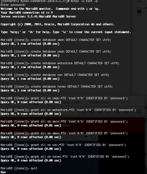
Cloudera Manager Installation
The following section describes installation of Cloudera Manager first and then using Cloudera Manager to install CDH 5.7.
Setting Up the Cloudera Manager Server Database
The Cloudera Manager Server Database stores information about service and host configurations.
Installing Cloudera Manager
Cloudera Manager, an end to end management application, is used to install and configure CDH. During CDH Installation, Cloudera Manager's Wizard will help to install Hadoop services on all nodes using the following procedure:
· Discovery of the cluster nodes
· Configure the Cloudera parcel or package repositories
· Install Hadoop, Cloudera Manager Agent (CMA) and Impala on all the cluster nodes.
· Install the Oracle JDK if it is not already installed across all the cluster nodes.
· Assign various services to nodes.
· Start the Hadoop services.
To install Cloudera Manager, complete the following steps:
1. Update the repo files to point to local repository.
#rm -f /var/www/html/clouderarepo/*.repo
#cp /etc/yum.repos.d/c*.repo /var/www/html/clouderarepo/
2. Install the Oracle Java Development Kit on the Cloudera Manager Server host.
3. #yum install oracle-j2sdk1.7
4. Install the Cloudera Manager Server packages either on the host where the database is installed, or on a host that has access to the database.
#yum install cloudera-manager-daemons cloudera-manager-server
Preparing a Cloudera Manager Server External Database
1. Run the scm_prepare_database.sh script on the host where the Cloudera Manager Server package is installed (rhel1) admin node.
#cd /usr/share/cmf/schema
#./scm_prepare_database.sh mysql amon root <password>
#./scm_prepare_database.sh mysql rman root <password>
#./scm_prepare_database.sh mysql metastore root <password>
#./scm_prepare_database.sh mysql nav root <password>
#./scm_prepare_database.sh mysql navms root <password>
#./scm_prepare_database.sh mysql sentry root <password>
#./scm_prepare_database.sh mysql oozie root <password>
2. Verify the database connectivity using the following command.
[root@rhel1 ~]# mysql –u root –p
mysql> connect amon
mysql> connect rman
mysql> connect metastore
mysql> connect nav
mysql> connect navms
mysql> connect sentry
mysql> connect oozie
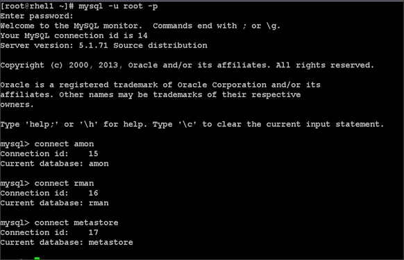
The MySQL External database setup is complete.
Starting The Cloudera Manager Server
1. Start the Coudera Manager Server
#service cloudera-scm-server start
2. Access the Cloudera Manager using the URL, http://10.4.1.31:7180 to verify that the server is up.
3. Once the installation of Cloudera Manager is complete, install CDH5 using the Cloudera Manager Web interface.
Installing Cloudera Enterprise Data Hub (CDH5)
To install the Cloudera Enterprise Data Hub, complete the following steps:
1. Login to the Cloudera Manager. Enter "admin" for both the Username and Password fields.
2. If you do not have a Cloudera license, select Cloudera Enterprise Data Hub Trial Edition. If you do have a Cloudera license, Click “Upload License” and select your license.
3. Based on requirement, choose appropriate Cloudera Editions for the Installation.
Figure 20 Installing Cloudera Enterprise
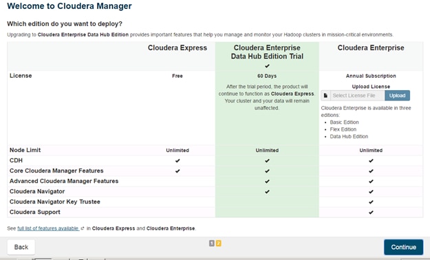
4. Click Continue on the confirmation page.
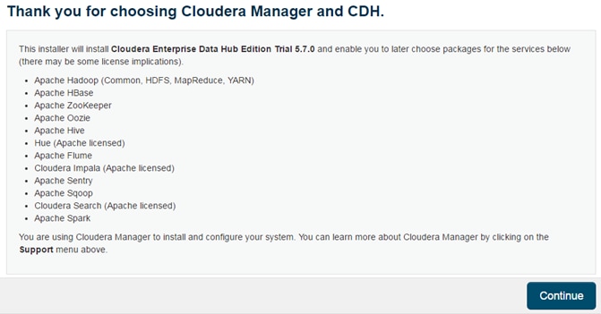
Edit the Cloudera Enterprise Parcel Settings to Use the CDH 5.7.0 Parcels
1. Open another tab in the same browser window and visit the URL: http://10.4.1.31:7180/cmf/parcel/status for modifying the parcel settings.
2. Click Configuration on this page.
3. Click to remove the entire remote repository URLs, and add the URL to the location where we kept the CDH 5.7.0 parcels i.e. http://10.4.1.31/CDH5.7parcels/.
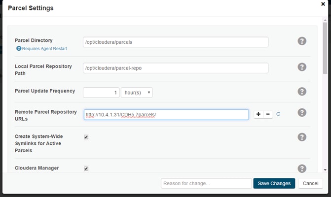
4. Click Save Changes to finish the configuration.
5. Navigate back to the Cloudera installation home page i.e. http://10.4.1.31:7180.
6. Click Continue on the confirmation page.

7. Specify the hosts that are part of the cluster using their IP addresses or hostname. The figure below shows use of a pattern to specify the IP addresses range.
10.4.1.[31-94] or rhel[1-64]
8. After the IP addresses or hostnames are entered, click Search.
Figure 21 Searching for Cluster Nodes
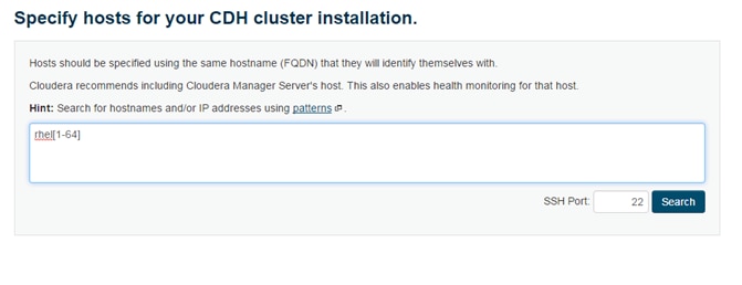
9. Cloudera Manager will "discover" the nodes in the cluster. Verify that all desired nodes have been found and selected for installation.
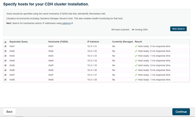
10. Click Continue.
11. For the method of installation, select the Use Parcels (Recommended) radio button.
12. For the CDH version, select the CDH5.7.0-1.cdh5.7.0.p0.45 radio button.
13. For the specific release of Cloudera Manager, select the Custom Repository radio button.
14. Enter the URL for the repository within the admin node. http://10.4.1.31/clouderarepo/cloudera-manager and click Continue.
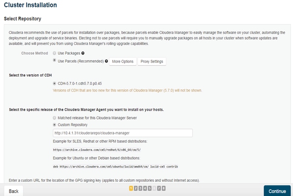
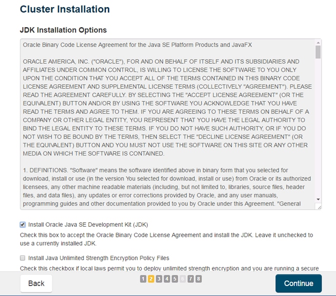
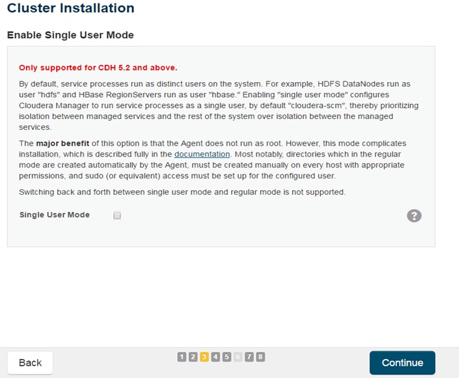
15. Provide SSH login credentials for the cluster and click Continue.
Figure 22 Login Credentials to Start CDH Installation
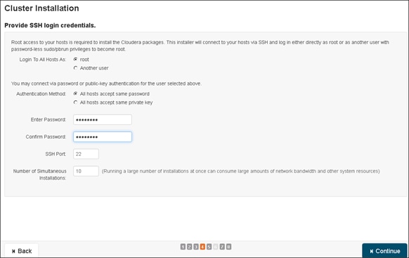
16. Installation using parcels begins.
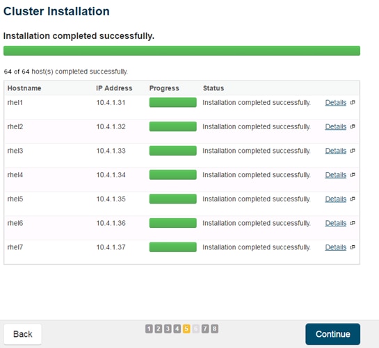
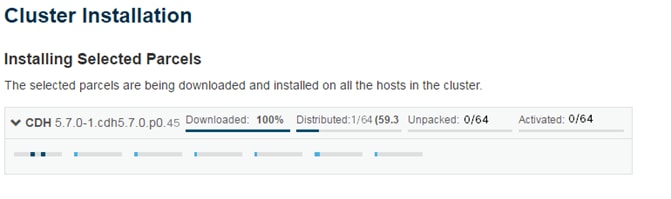
17. Once the installation is completed successfully, click Continue to select the required services.
18. Wait for Cloudera Manager to inspect the hosts on which it has just performed the installation.
19. Review and verify the summary. Click Continue.
Figure 23 Inspecting Hosts for Correctness
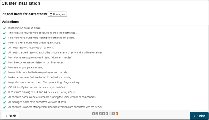
20. Select services that need to be started on the cluster.
Figure 24 Selecting CDH Version and Services
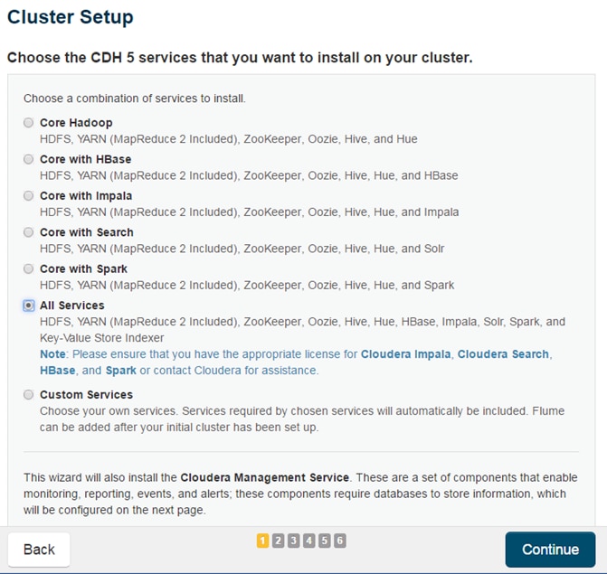
21. This is one of the critical steps in the installation. Inspect and customize the role assignments of all the nodes based on your requirements and click Continue.
22. Reconfigure the service assignment to match Table 8 below.
| Service Name |
Host |
| NameNode |
rhel1, rhel2 (HA) |
| HistoryServer |
rhel1 |
| JournalNodes |
rhel1,rhel2,rhel3 |
| ResouceManager |
rhel2, rhel3(HA) |
| Hue Server |
rhel2 |
| HiveMetastore Server |
rhel1 |
| HiveServer2 |
rhel2 |
| HBase Master |
rhel2 |
| Oozie Server |
rhel1 |
| ZooKeeper |
rhel1, rhel2, rhel3 |
| DataNode |
rhel4 to rhel64 |
| NodeManager |
rhel4 to rhel64 |
| RegionServer |
rhel4 to rhel64 |
| Sqoop Server |
rhel1 |
| Impala Catalog Server Daemon |
rhel1 |
| Impala State Store |
rhel2 |
| Impala Daemon |
rhel4 to rhel64 |
| Solr Server |
rhel4( can be installed on all hosts if needed, if there is a search use case) |
| Spark History Server |
rhel1 |
| Spark Executors |
rhel4 to rhel64 |
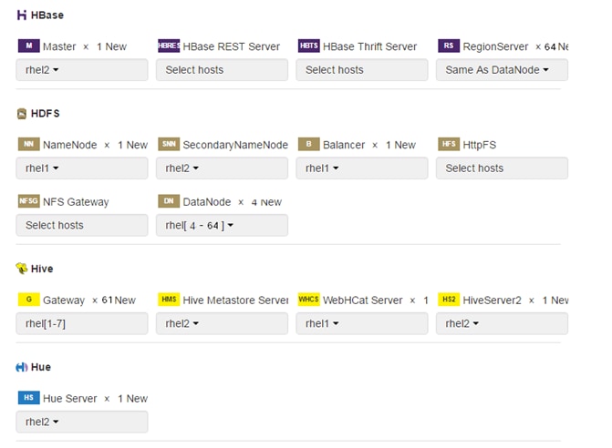
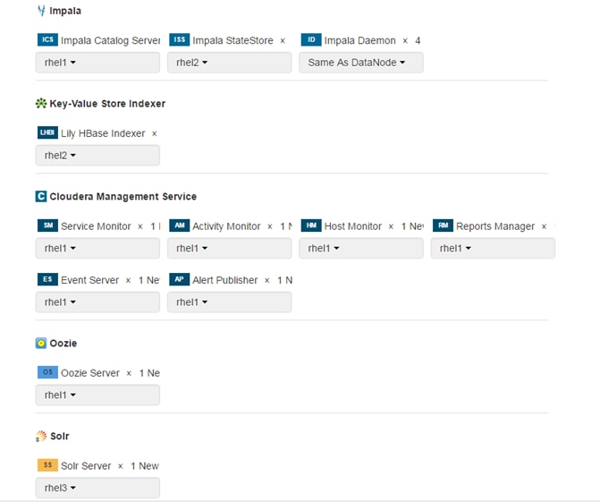
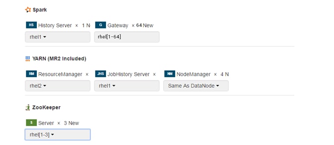
Setting up the Database
The role assignment recommendation above is for clusters of up to 64 servers. For clusters larger than 64 nodes, use the HA recommendation defined in Table 8 above.
1. In the Database Host Name sections use port 3306 for TCP/IP because connection to the remote server always uses TCP/IP.
2. Enter the Database Name, username and password that were used during the database creation stage earlier in this document.
3. Click Test Connection to verify the connection and click Continue.
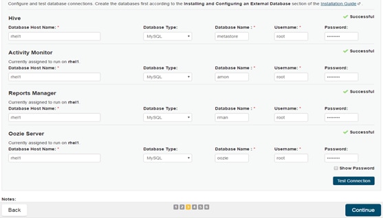
4. Review and customize the configuration changes based on your requirements.
Figure 26 Review the Configuration Changes Part1
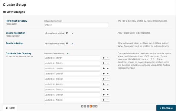
5. Click Continue to start running the cluster services.
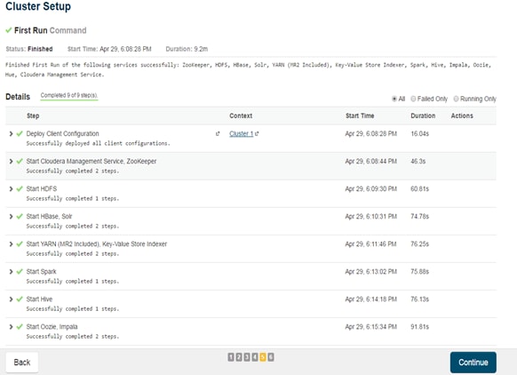
Starting the Cluster Services
1. Hadoop services are installed, configured and now running on all the nodes of the cluster. Click Finish to complete the installation.
Figure 27 Installation Completion
Cloudera Manager now displays the status of all Hadoop services running on the cluster.
Figure 28 Service Status of the Cluster
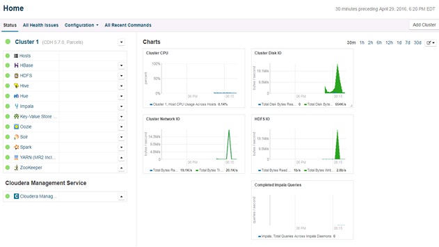
Scaling the Cluster
The role assignment recommendation above is for cluster with at least 64 servers and in High Availability (HA). For smaller cluster running without HA the recommendation is to dedicate one server for NameNode and a second server for secondary name node and YARN Resource Manager. For larger clusters larger than 64 nodes the recommendation is to dedicate one server each for name node, YARN Resource Manager and one more for running both NameNode (HA) and Resource Manager (HA) as in the table (no Secondary NameNode when in HA).
For production clusters it is recommended to set up NameNode and Resource manager in HA mode.
This implies that there will be at least 3 master nodes, running the NameNode, YARN Resource manager, the failover counter-part being designated to run on another node and a third node that would have similar capacity as the other two nodes.
All the three nodes will also need to run zookeeper and quorum journal node services. It is also recommended to have a minimum of 5 DataNodes in a cluster. Please refer to the next section for details on how to enable HA.
Enabling High Availability
![]() Note: Setting up HA is done after the Cloudera Installation is completed.
Note: Setting up HA is done after the Cloudera Installation is completed.
HDFS High Availability
The HDFS HA feature provides the option of running two NameNodes in the same cluster, in an Active/Passive configuration. These are referred to as the Active NameNode and the Standby NameNode. Unlike the Secondary NameNode, the Standby NameNode is a hot standby, allowing a fast failover to a new NameNode in the case that a machine crashes, or a graceful administrator-initiated failover for the purpose of planned maintenance. There cannot be more than two NameNodes.
For more information go to:
Setting Up HDFS HA
The Enable High Availability workflow leads through adding a second (standby) NameNode and configuring JournalNodes. During the workflow, Cloudera Manager creates a federated namespace.
1. Log in to the admin node (rhel1) and create the Edit directory for the JournalNode
#clush -w rhel[1-3] mkdir -p /data/disk1/namenode-edits
#clush -w rhel[1-3] chmod 777 /data/disk1/namenode-edits
![]()
2. Log in to the Cloudera manager and go to the HDFS service.
3. In the top right corner Select Actions> Enable High Availability. A screen showing the hosts that are eligible to run a standby NameNode and the JournalNodes displays.
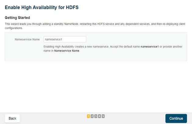
4. Specify a name for the nameservice or accept the default name nameservice1 and click Continue.
5. In the NameNode Hosts field, click Select a host. The host selection dialog displays.
6. Check the checkbox next to the hosts (rhel2) where the standby NameNode is to be set up and click OK.
![]() Note: The standby NameNode cannot be on the same host as the active NameNode, and the host that is chosen should have the same hardware configuration (RAM, disk space, number of cores, and so on) as the active NameNode.
Note: The standby NameNode cannot be on the same host as the active NameNode, and the host that is chosen should have the same hardware configuration (RAM, disk space, number of cores, and so on) as the active NameNode.
7. In the JournalNode Hosts field, click Select hosts. The host selection dialog displays.
8. Check the checkboxes next to an odd number of hosts (a minimum of three) to act as JournalNodes and click OK. Here we are using the same nodes as Zookeeper nodes.
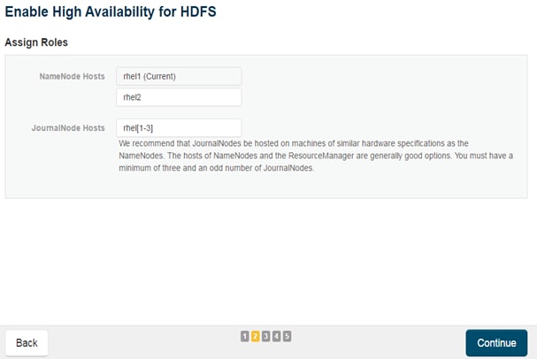
![]() Note: JournalNodes should be hosted on hosts with similar hardware specification as the NameNodes. It is recommended that each JournalNode is put on the same hosts as the active and standby NameNodes, and the third JournalNode on ResourceManager node.
Note: JournalNodes should be hosted on hosts with similar hardware specification as the NameNodes. It is recommended that each JournalNode is put on the same hosts as the active and standby NameNodes, and the third JournalNode on ResourceManager node.
9. Click Continue.
10. In the JournalNode Edits Directory property, enter a directory location created earlier in step 1 for the JournalNode edits directory into the fields for each JournalNode host.
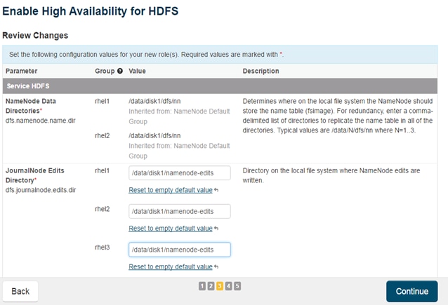
![]() Note: The directories specified should be empty, and must have the appropriate permissions.
Note: The directories specified should be empty, and must have the appropriate permissions.
Extra Options: Decide whether Cloudera Manager should clear existing data in ZooKeeper, Standby NameNode, and JournalNodes. If the directories are not empty (for example, re-enabling a previous HA configuration), Cloudera Manager will not automatically delete the contents—select to delete the contents by keeping the default checkbox selection. The recommended default is to clear the directories.
![]() Note: If chosen not to do so, the data should be in sync across the edits directories of the JournalNodes and should have the same version data as the NameNodes.
Note: If chosen not to do so, the data should be in sync across the edits directories of the JournalNodes and should have the same version data as the NameNodes.
11. Click Continue.
Cloudera Manager executes a set of commands that will stop the dependent services, delete, create, and configure roles and directories as appropriate, create a nameservice and failover controller, and restart the dependent services and deploy the new client configuration.
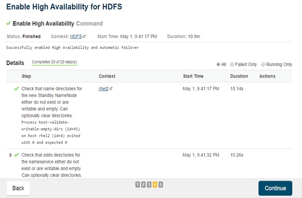
![]() Note: Formatting of name directory is expected to fail, if the directories are not empty.
Note: Formatting of name directory is expected to fail, if the directories are not empty.
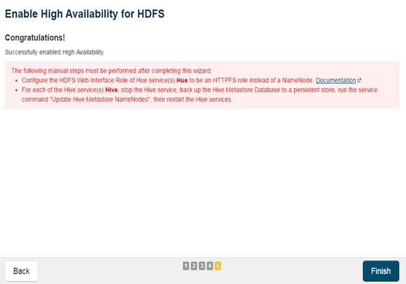
12. In the next screen additional steps are suggested by the Cloudera Manager to update the Hue and Hive metastore. Click finish for the screen shown above.
![]() Note: The following subsections cover configuring Hue and Hive for HA as needed.
Note: The following subsections cover configuring Hue and Hive for HA as needed.
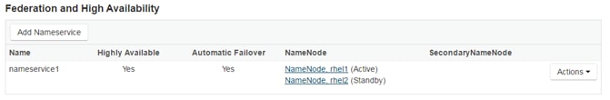
13. In the Cloudera Manager, Click on Home> HDFS> Instances to see Namenode in High Availability.
Configuring Hive Metastore to Use HDFS HA
The Hive metastore can be configured to use HDFS high availability.
1. Go the Hive service.
2. Select Actions> Stop.
3. Click Stop to confirm the command.
4. Back up the Hive metastore database (if any existing data is present)
5. Select Actions> Update Hive Metastore NameNodes and confirm the command.
6. Select Actions> Start.
7. Restart the Hue and Impala services if stopped prior to updating the Metastore.
Configuring Hue to Work with HDFS HA
1. Go to the HDFS service.
2. Click the Instances tab.
3. Click Add Role Instances.
4. Select the text box below the HttpFS field. The Select Hosts dialog displays.
5. Select the host on which to run the role and click OK.
6. Click Continue.
7. Check the checkbox next to the HttpFS role and select Actions for Selected> Start.
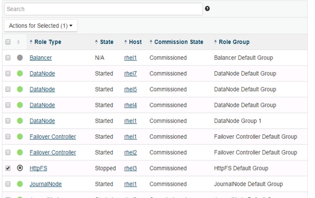
8. After the command has completed, go to the Hue service.
9. Click the Configuration tab.
10. Locate the HDFS Web Interface Role property or search for it by typing its name in the Search box.
11. Select the HttpFS role that was just created instead of the NameNode role, and save your changes.
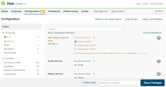
12. Restart the Hue service.
![]() Note: Refer to the Cloudera website: http://www.cloudera.com/documentation/enterprise/5-3-x/topics/cdh_hag_hdfs_ha_cdh_components_config.html - concept_rj1_hsq_bp for further details on setting up HA for other components like Impala, Oozie etc.
Note: Refer to the Cloudera website: http://www.cloudera.com/documentation/enterprise/5-3-x/topics/cdh_hag_hdfs_ha_cdh_components_config.html - concept_rj1_hsq_bp for further details on setting up HA for other components like Impala, Oozie etc.
YARN High Availability
The YARN Resource Manager (RM) is responsible for tracking the resources in a cluster and scheduling applications (for example, MapReduce jobs). Before CDH 5, the RM was a single point of failure in a YARN cluster. The RM high availability (HA) feature adds redundancy in the form of an Active/Standby RM pair to remove this single point of failure. Furthermore, upon failover from the Standby RM to the Active, the applications can resume from their last check-pointed state; for example, completed map tasks in a MapReduce job are not re-run on a subsequent attempt. This allows events such the following to be handled without any significant performance effect on running applications.
· Unplanned events such as machine crashes.
· Planned maintenance events such as software or hardware upgrades on the machine running the ResourceManager
For more information please go to: http://www.cloudera.com/documentation/enterprise/latest/topics/cdh_hag_rm_ha_config.html - xd_583c10bfdbd326ba--43d5fd93-1410993f8c2--7f77
Setting up YARN HA
1. Log in to the Cloudera manager and go to the YARN service.
2. Select Actions> Enable High Availability.
A screen showing the hosts that are eligible to run a standby ResourceManager displays.
The host where the current ResourceManager is running is not available as a choice.
3. Select the host (rhel3) where the standby ResourceManager is to be installed, and click Continue.
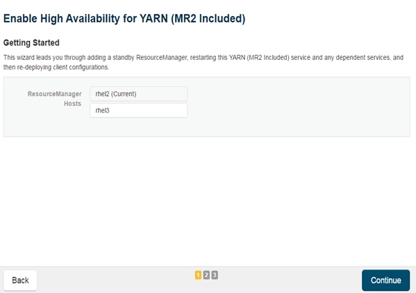
Cloudera Manager proceeds to execute a set of commands that stop the YARN service, add a standby ResourceManager, initialize the ResourceManager high availability state in ZooKeeper, restart YARN, and redeploy the relevant client configurations.
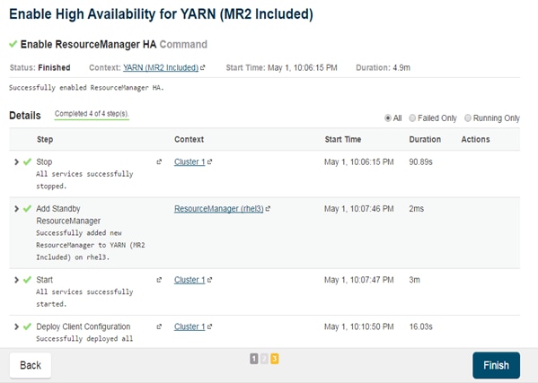
4. Click Finish once the installation is completed successfully.
Configuring Yarn (MR2 Included) and HDFS Services
The parameters in Table 9 are used for Cisco UCS Integrated Infrastructure for Big Data and Analytics Performance Optimized cluster configuration described in this document. These parameters are to be changed based on the cluster configuration, number of nodes and specific workload.
| Service |
Value |
| mapreduce.map.memory.mb |
3GiB |
| mapreduce.reduce.memory.mb |
3GiB |
| mapreduce.map.java.opts.max.heap |
2560 MiB |
| yarn.nodemanager.resource.memorymb |
180 GiB |
| yarn.nodemanager.resource.cpu-vcores |
32 |
| yarn.scheduler.minimum-allocation-mb |
4 GiB |
| yarn.scheduler.maximum-allocation-mb |
180 GiB |
| yarn.scheduler.maximum-allocation-vcores |
48 |
| mapreduce.task.io.sort.mb |
256 MiB |
Table 10 HDFS
| dfs.datanode.failed.volumes.tolerated |
6 |
| dfs.datanode.du.reserved |
50 GiB |
| dfs.datanode.data.dir.perm |
755 |
| Java Heap Size of Namenode in Bytes |
2628 MiB |
| dfs.namenode.handler.count |
54 |
| dfs.namenode.service.handler.count |
54 |
| Java Heap Size of Secondary namenode in Bytes |
2628 MiB |
Apache Kafka Installation and Configuration
Cloudera Manager 5.4 or higher includes the Kafka service. To install, download Kafka using Cloudera Manager, distribute Kafka to the cluster, activate the new parcel, and add the service to the cluster.
1. Download the Kafka Parcels as shown below.
2. On a server that is accessible to the internet.
3. Create a directory for the Kakfa parcels
#mkdir /tmp/Kafka2.0.1Parcels
#cd /tmp/Kafka2.0.1Parcels
#wget http://archive.cloudera.com/kafka/parcels/2.0.1/KAFKA-2.0.1-1.2.0.1.p0.5-el7.parcel
#wget http://archive.cloudera.com/kafka/parcels/2.0.1/KAFKA-2.0.1-1.2.0.1.p0.5-el7.parcel.sha1
#wget http://archive.cloudera.com/kafka/parcels/2.0.1/manifest.json
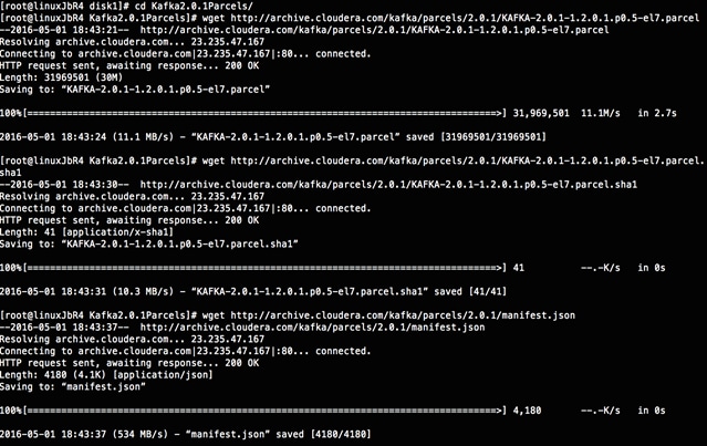
4. Change the contents of manifest.json to match the following
{
"lastUpdated": 14598141460000,
"parcels": [
{
"parcelName": "KAFKA-2.0.1-1.2.0.1.p0.5-el7.parcel",
"components": [
{
"pkg_version": "0.9.0+kafka2.0.1",
"pkg_release": "1.2.0.1.p0.5",
"name": "kafka",
"version": "0.9.0-kafka2.0.1"
}
],
"depends": "CDH (>= 5.2), CDH (<< 6.0)",
"replaces": "CLABS_KAFKA",
"hash": "180d8322f2026f2b3609741216d2c25dd2dfb294"
}
]
}
5. Copy the Kafka parcels over to rhel1 under /var/www/html
#scp -r Kafka2.0.1Parcels rhel1:/var/www/html/
6. From the browser go to the parcels at http://10.4.1.31:7180/cmf/parcel/status.
7. Click on configure. Add in a new parcel by clicking on the + button and giving the path to the new Kafka parcels that were downloaded in the previous step.
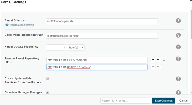
8. Click on Save Changes.
9. Click Download and then Distribute to download and distribute the parcels.
10. Click Activate to add the service to the cluster.
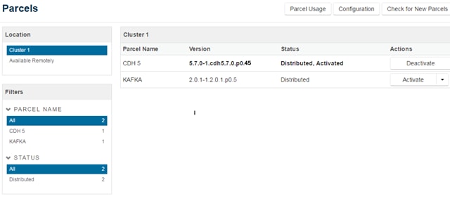
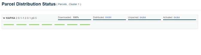
Once Activation is complete the Kafka service is ready to be installed on the Cluster.
Kafka Installation
1. Click on the arrow next to the Cluster Name and Select Add A Service.
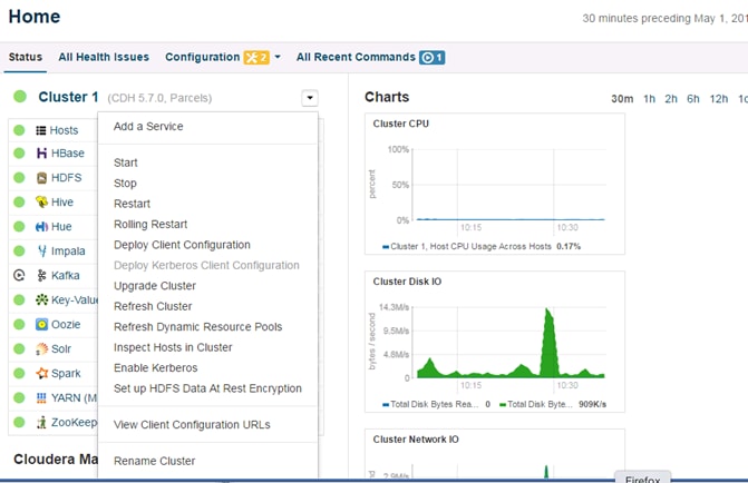
2. This shows all the available services. Select Kafka from the list.
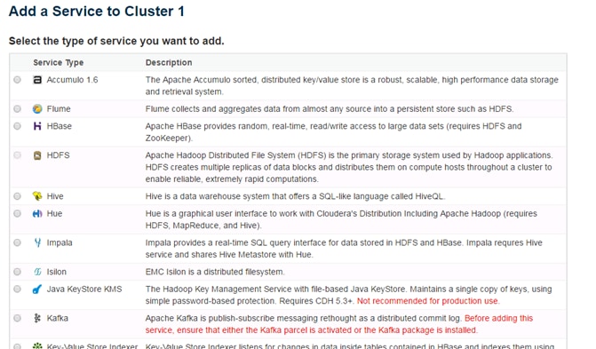
3. Click Continue to go ahead with the installation.
4. Select the hosts on which Kafka Broker(s) needs to be enabled. In this CVD Kafka is enabled only on two nodes.
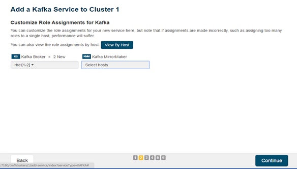
5. The Default Replication Factor in Kafka is 1; change that to 3 and click on Continue to enable the services.
![]() Note: Kafka MirrorMaker is needed for when dealing with multiple Kafka clusters to replicate data across data centers.
Note: Kafka MirrorMaker is needed for when dealing with multiple Kafka clusters to replicate data across data centers.
6. Change the broker_max_heap_size to 512MB.
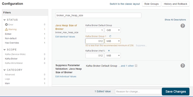
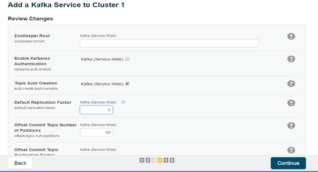
7. Click on Continue to start the service.
Kafka works well for smaller messages, the best performance occurs with 1 KB messages. Please go to the link below for further Performance and Resource tuning configurations for Kafka: http://www.cloudera.com/documentation/kafka/latest/topics/kafka_performance.html
Configuring Spark
The two main resources that Spark (and YARN) are dependent on are CPU and memory. Disk and network I/O, of course, play a part in Spark performance as well, but neither Spark nor YARN currently can actively manage them. Every Spark executor in any application has the same fixed number of cores and same fixed heap size. The number of cores can be specified with the executor-cores flag when invoking spark-submit, spark-shell, and pyspark from the command line, or by setting the spark.executor.cores property in the spark-defaults.conf file or in the SparkConf object.
And the heap size can be controlled with the executor-memory flag or the spark.executor.memory property. The cores property controls the number of concurrent tasks an executor can run, executor-cores = 5 mean that each executor can run a maximum of five tasks at the same time. The memory property impacts the amount of data Spark can cache, as well as the maximum sizes of the shuffle data structures used for grouping, aggregations, and joins.
The num-executors command-line flag or spark.executor.instances configuration property control the number of executors requested. Dynamic Allocation can be enabled from CDH5.4 instead setting the spark.dynamicAllocation.enabled to true. Dynamic allocation enables a Spark application to request executors when there is a backlog of pending tasks and free up executors when idle.
Asking for five executor cores will result in a request to YARN for five virtual cores. The memory requested from YARN is a little more complex for a couple reasons:
· executor-memory/spark.executor.memory controls the executor heap size, but JVMs can also use some memory off heap, for example for VM overhead, interned Strings and direct byte buffers. The value of the spark.yarn.executor.memoryOverhead property is added to the executor memory to determine the full memory request to YARN for each executor. It defaults to max (384, 0.10 * spark.executor.memory).
· YARN may round the requested memory up a little. YARN’s yarn.scheduler.minimum-allocation-mb and yarn.scheduler.increment-allocation-mb properties control the minimum and increment request values respectively.
· The application master is a non-executor container with the special capability of requesting containers from YARN, takes up resources of its own that must be budgeted in. In yarn-client mode, it defaults to a 1024MB and one vcore. In yarn-cluster mode, the application master runs the driver, so it’s often useful to add its resources with the –driver-memory and –driver-cores properties.
· Running executors with too much memory often results in excessive garbage collection delays. 64GB is a rough guess at a good upper limit for a single executor.
· A good estimate is that at most five tasks per executor can achieve full write throughput, so it’s good to keep the number of cores per executor around that number.
· Running tiny executors (with a single core and just enough memory needed to run a single task, for example) throws away the benefits that come from running multiple tasks in a single JVM. For example, broadcast variables need to be replicated once on each executor, so many small executors will result in many more copies of the data.
Tuning Resource Allocation for Spark
Below is an example of configuring a Spark application to use as much of the cluster as possible, we are using an example cluster with 16 nodes running NodeManagers, each equipped with 56 cores and 256GB of memory. yarn.nodemanager.resource.memory-mb and yarn.nodemanager. resource.cpu-vcores should be set to 180 * 1024 = 184320 (megabytes) and 48 respectively.
spark.executor.instances/num-executors = 63
spark.executor.cores/--executor-cores = 5
spark.executor.memory/--executor-memory = 41G
This configuration results in four executors on all nodes except for the one with the AM, which will have three executors.
executor-memory is derived as (180/4 executors per node) = 45; 45 * 0.10 = 4.5 45 – 4.5 ~ 40.
For taking care of long running processes use 2G for the spark driver:
spark.driver.memory = 2G
For submitting a job
--driver -memory 2G –executor -memory 40G --num-executors 63 --executor-cores 5 --properties-file /opt/cloudera/parcels/CDH/etc/spark/conf.dist/spark-defaults.conf
In yarn-cluster mode, the local directories used by the Spark executors and the Spark driver will be the local directories configured for YARN (Hadoop YARN config yarn.nodemanager.local-dirs). If the user specifies spark.local.dir, it will be ignored.
In yarn-client mode, the Spark executors will use the local directories configured for YARN while the Spark driver will use those defined in spark.local.dir. The Spark driver does not run on the YARN cluster in yarn-client mode, only the Spark executors do.
spark.local.dir /tmp (Directory to use for "scratch" space in Spark, including map output files and RDDs that get stored on disk. This should be on a fast, local disk in your system).
Every Spark stage has a number of tasks, each of which processes data sequentially. In tuning Spark jobs, this parallelism number is the most important parameter in determining performance. The number of tasks in a stage is the same as the number of partitions in the last RDD in the stage. The number of partitions in an RDD is the same as the number of partitions in the RDD on which it depends, with a couple exceptions: the coalesce transformation allows creating an RDD with fewer partitions than its parent RDD, the union transformation creates an RDD with the sum of its parents’ number of partitions, and Cartesian creates an RDD with their product.
RDDs produced by a file have their partitions determined by the underlying MapReduce InputFormat that’s used. Typically there will be a partition for each HDFS block being read. Partitions for RDDs produced by parallelize come from the parameter given by the user, or spark.default.parallelism if none is given.
The primary concern is that the number of tasks will be too small. If there are fewer tasks than slots available to run them in, the stage won’t be taking advantage of all the CPU available.
If the stage in question is reading from Hadoop, your options are:
· Use the repartition transformation, which will trigger a shuffle.
· Configure your InputFormat to create more splits.
· Write the input data out to HDFS with a smaller block size.
If the stage is getting its input from another stage, the transformation that triggered the stage boundary will accept a numPartitions argument.
The most straightforward way to tune the number of partitions is experimentation: Look at the number of partitions in the parent RDD and then keep multiplying that by 1.5 until performance stops improving.
In contrast with MapReduce for Spark when in doubt, it’s almost always better to be on the side of a larger number of tasks (and thus partitions).
Shuffle performance improvement
spark.shuffle.compress true (compress map output files)
spark.broadcast.compress true(compress broadcast variables before sending them)
spark.io.compression.codec org.apache.spark.io.SnappyCompressionCodec (codec used to compress internal data such as RDD partitions, broadcast variables and shuffle outputs)
spark.shuffle.spill.compress true (Whether to compress data spilled during shuffles.)
spark.shuffle.io.numConnectionsPerPeer 4 (Connections between hosts are reused in order to reduce connection buildup for large clusters. For clusters with many hard disks and few hosts, this may result in insufficient concurrency to saturate all disks, and so users may consider increasing this value.)
spark.shuffle.file.buffer 64K (Size of the in-memory buffer for each shuffle file output stream. These buffers reduce the number of disk seeks and system calls made in creating intermediate shuffle file)
Improving Serialization performance
Serialization plays an important role in the performance of any distributed application. Often, this will be the first thing that should be tuned to optimize a Spark application.
spark.serializer org.apache.spark.serializer.KryoSerializer (when speed is necessary)
spark.kryo.referenceTracking false
spark.kryoserializer.buffer 2000 (If the objects are large, may need to increase the size further to fit the size of the object being deserialized).
SparkSQL is ideally suited for mixed procedure jobs where SQL code is combined with Scala, Java, or Python programs. In general the SparkSQL command line interface is used for single user operations and ad hoc queries.
For multi-user SparkSQL environments, it is recommended to use a Thrift server connected via JDBC.
Spark SQL Tuning
Below are some guidelines for Spark SQL tuning.
1. To compile each query to Java bytecode on the fly, turn on sql.codegen. This can improve performance for large queries, but can slow down very short queries.
spark.sql.codegen true
spark.sql.unsafe.enabled true
2. Configuration of in-memory caching can be done using the setConf method on SQLContext or by running SET key=value commands using SQL.
3. spark.sql.inMemoryColumnarStorage.compressed true (will automatically select a compression codec for each column based on statistics of the data)
4. spark.sql.inMemoryColumnarStorage.batchSize 5000 (Controls the size of batches for columnar caching. Larger batch sizes can improve memory utilization and compression, but risk OOMs when caching data)
5. The columnar nature of the ORC format helps avoid reading unnecessary columns, but it is still possible to read unnecessary rows. ORC avoids this type of overhead by using predicate push-down with three levels of built-in indexes within each file: file level, stripe level, and row level. This combination of indexed data and columnar storage reduces disk I/O significantly, especially for larger datasets where I/O bandwidth becomes the main bottleneck for performance.
6. By default, ORC predicate push-down is disabled in Spark SQL. To obtain performance benefits from predicate push-down, enable it explicitly, as follows:
7. spark.sql.orc.filterPushdown=true
8. In SparkSQL to automatically determine the number of reducers for joins and groupbys, use the parameter,
9. spark.sql.shuffle.partitions 200, (default value is 200)
This property can be put into hive-site.xml to override the default value.
10. Set log to WARN in log4j.properties to reduce log level.
![]() Note: Running Thrift server and connecting to spark-sql through beeline is the recommended option for multi-session testing.
Note: Running Thrift server and connecting to spark-sql through beeline is the recommended option for multi-session testing.
Compression for Hive
1. Set the following Hive parameters to compress the Hive output files using Snappy compression:
hive.exec.compress.output=true
hive.exec.orc.default.compress=SNAPPY
Changing the Log Directory for All Applications
To change the default log from the /var prefix to /data/disk1, complete the following steps:
1. Log into the cloudera home page and click my clusters.
2. From the configuration drop down menu select “All Log Directories”
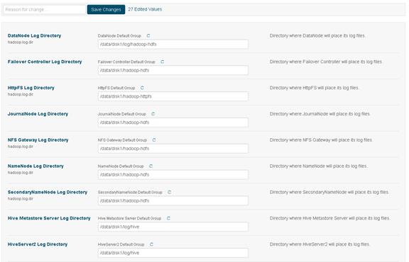
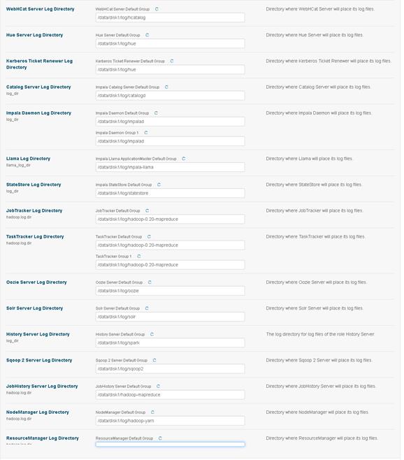
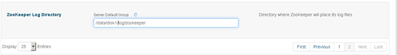
3. Click Save changes.
This section provides the BOM for the 64 nodes Performance Optimized Cluster. See Table 11 for BOM for the master rack, Table 12 for BOM for expansion racks (racks 2 to 4), Table 13 and Table 14 for software components. Table 15 lists Cloudera SKUs available from Cisco.
![]() If UCSD-SL-CPA4-P2 is added to the BOM all the required components for 16 servers only are automatically added. If not customers can pick each of the individual components that are specified after this and build the BOM manually.
If UCSD-SL-CPA4-P2 is added to the BOM all the required components for 16 servers only are automatically added. If not customers can pick each of the individual components that are specified after this and build the BOM manually.
Table 11 Bill of Materials for C240M4SX Base Rack
![]() If using the FI 6332 please refer to Table 1 for the SKU information.
If using the FI 6332 please refer to Table 1 for the SKU information.
Table 12 Bill of Materials for Expansion Racks
Table 13 Red Hat Enterprise Linux License
| Red Hat Enterprise Linux |
||
| RHEL-2S2V-3A |
Red Hat Enterprise Linux |
64 |
| CON-ISV1-EL2S2V3A |
3 year Support for Red Hat Enterprise Linux |
64 |
| Cloudera Software edition needed for this CVD |
||
| Cloudera Enterprise Flex Edition |
UCS-BD-CEDHC-BZ= |
64 |
| Cloudera Enterprise Data Hub Edition |
UCS-BD-CEDHC-GD= |
64 |
Table 15 Cloudera SKU’s available at Cisco
| Cisco TOP SKU |
Cisco PID with Duration |
Product Name |
| UCS-BD-CEBN-BZ= |
UCS-BD-CEBN-BZ-3Y |
Cloudera Enterprise Basic Edition, Node License, Bronze Support - 3 Year |
| UCS-BD-CEBN-BZI= |
UCS-BD-CEBN-BZI-3Y |
Cloudera Enterprise Basic Edition + Indemnification, Node License, Bronze Support - 3 Year |
| UCS-BD-CEBN-GD= |
UCS-BD-CEBN-GD-3Y |
Cloudera Enterprise Basic Edition, Node License, Gold Support - 3 Year |
| UCS-BD-CEBN-GDI= |
UCS-BD-CEBN-GDI-3Y |
Cloudera Enterprise Basic Edition + Indemnification, Node License, Gold Support - 3 Year |
| UCS-BD-CEDEN-BZ= |
UCS-BD-CEDEN-BZ-3Y |
Cloudera Enterprise Data Engineering Edition, Node License, Bronze Support - 3 Year |
| UCS-BD-CEDEN-GD= |
UCS-BD-CEDEN-GD-3Y |
Cloudera Enterprise Data Engineering Edition, Node License, Gold Support - 3 Year |
| UCS-BD-CEODN-BZ= |
UCS-BD-CEODN-BZ-3Y |
Cloudera Enterprise Operational Database Edition, Node License, Bronze Support - 3 Year |
| UCS-BD-CEODN-GD= |
UCS-BD-CEODN-GD-2Y |
Cloudera Enterprise Operational Database Edition, Node License, Gold Support - 2 Year |
| UCS-BD-CEODN-GD= |
UCS-BD-CEODN-GD-3Y |
Cloudera Enterprise Operational Database Edition, Node License, Gold Support - 3 Year |
| UCS-BD-CEADN-BZ= |
UCS-BD-CEADN-BZ-3Y |
Cloudera Enterprise Analytical Database Edition, Node License, Bronze Support - 3 Year |
| UCS-BD-CEADN-GD= |
UCS-BD-CEADN-GD-3Y |
Cloudera Enterprise Analytical Database Edition, Node License, Gold Support - 3 Year |
| UCS-BD-CEDHN-BZ= |
UCS-BD-CEDHN-BZ-3Y |
Cloudera Enterprise Data Hub Edition, Node License, Bronze Support - 3 Year |
| UCS-BD-CEDHN-GD= |
UCS-BD-CEDHN-GD-3Y |
Cloudera Enterprise Data Hub Edition, Node License, Gold Support - 3 Year |
| UCS-BD-CEBC-BZ= |
UCS-BD-CEBC-BZ-3Y |
Cloudera Enterprise Basic Edition, Capacity License, Bronze Support - 3 Year |
| UCS-BD-CEBC-BZI= |
UCS-BD-CEBC-BZI-3Y |
Cloudera Enterprise Basic Edition + Indemnification, Capacity License, Bronze Support - 3 Year |
| UCS-BD-CEBC-GD= |
UCS-BD-CEBC-GD-3Y |
Cloudera Enterprise Basic Edition, Capacity License, Gold Support - 3 Year |
| UCS-BD-CEBC-GDI= |
UCS-BD-CEBC-GDI-3Y |
Cloudera Enterprise Basic Edition + Indemnification, Capacity License, Gold Support - 3 Year |
| UCS-BD-CEDEC-BZ= |
UCS-BD-CEDEC-BZ-3Y |
Cloudera Enterprise Data Engineering Edition, Capacity License, Bronze Support - 3 Year |
| UCS-BD-CEDEC-GD= |
UCS-BD-CEDEC-GD-3Y |
Cloudera Enterprise Data Engineering Edition, Capacity License, Gold Support - 3 Year |
| UCS-BD-CEODC-BZ= |
UCS-BD-CEODC-BZ-3Y |
Cloudera Enterprise Operational Database Edition, Capacity License, Bronze Support - 3 Year |
| UCS-BD-CEODC-GD= |
UCS-BD-CEODC-GD-3Y |
Cloudera Enterprise Operational Database Edition, Capacity License, Gold Support - 3 Year |
| UCS-BD-CEADC-BZ= |
UCS-BD-CEADC-BZ-3Y |
Cloudera Enterprise Analytical Database Edition, Capacity License, Bronze Support - 3 Year |
| UCS-BD-CEADC-GD= |
UCS-BD-CEADC-GD-3Y |
Cloudera Enterprise Analytical Database Edition, Capacity License, Gold Support - 3 Year |
| UCS-BD-CEDHC-BZ= |
UCS-BD-CEDHC-BZ-3Y |
Cloudera Enterprise Data Hub Edition, Capacity License, Bronze Support - 3 Year |
| UCS-BD-CEDHC-GD= |
UCS-BD-CEDHC-GD-3Y |
Cloudera Enterprise Data Hub Edition, Capacity License, Gold Support - 3 Year |
Chinmayi Narasimhadevara, Big Data Software Engineer, Data Center Solutions Group, Cisco Systems, Inc. Chinmayi's focus areas are solutions and emerging trends in Big Data and analytics related technologies and infrastructure in the Data Center.
Acknowledgements
· Manan Trivedi, Big Data Solutions Engineer, Data Center Solutions Group, Cisco Systems Inc.
· Karthik Kulkarni, Big Data Solutions Architect, Data Center Solutions Group, Cisco Systems Inc.
· Mo Jamal, Solutions Architect at Cloudera
· Dwai Lahari, Solutions Architect at Cloudera.
· Alex Moundalexis, Senior Solutions Architect at Cloudera
· Barbara Dixon, Technical Writer, Data Center Solutions Group, Cisco Systems, Inc.
Setting Up Network Bonding
Network bonding can be setup on the vNICs on the hosts for redundancy as well as for increased throughput. Below is example of how bonding can be configured on a 16-node cluster.
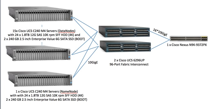
Enabling bonding will need the Fabric Interconnects to connect to any L2/L3 switch in this example the N9K-9372PX switch is used. All the ports that will be used will need to be bundled in a port channel. In this example we bundled 8 ports into the port channel. In this configuration 3 vNICs are used on each FI, while one vNIC on each is sufficient the reason for this is multiple vNIC bonding works much better with bonding mode 6, because both sending and receiving frames are load balanced with different MAC addresses.
By the very definition of bond mode 6 (balance-alb),“when a link is reconnected or a new slave joins the bond the received traffic is redistributed among all active slaves in the bond by initiating ARP Replies with the selected MAC address to each of the clients.” This explains the performance improvement that is observed with addition of multiple vNICS.
VLANs are configured as shown in Table 16 below:
| VLAN |
Fabric |
NIC Port |
Function |
| Vlan19 |
|
bond0 |
Data |
|
|
A |
eth0 |
Data |
|
|
B |
eth1 |
Data |
|
|
A |
eth2 |
Data |
|
|
B |
eth3 |
Data |
|
|
A |
eth4 |
Data |
|
|
B |
eth5 |
Data |
All NICs are carrying data traffic in Vlan19.
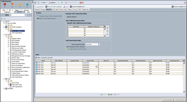
16 upstream ports bundled in Port channel created between Fabric Interconnect and upstream switch (Nexus N9K-C9372PX)
1. Configure eth0 as shown below and click on Apply to enable the changes.
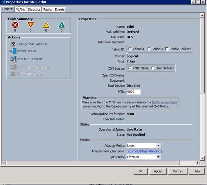
All vNICs (eth0-eth5) are the same as the above configuration. The only change will be the Fabric ID as noted below:
· eth0, eth2, and eth4 are on the link going to Fabric A
· eth1, eth3, and eth5 are on the link going to Fabric B
· All 6 vNICs are bonded together in Mode 6 to form bond0 interface.
To configure bonding on the OS Host machines, complete the following steps:
1. Configure /etc/modules.conf as follows:
alias bond0 bonding
Sample ifcfg-eth0 file
DEVICE="eth0"
BOOTPROTO="none"
MTU="9000"
ONBOOT="yes"
TYPE="Ethernet"
MASTER=bond0
SLAVE=yes
2. All the vNICs that are being bonded will need to be configured as SLAVES as shown above on all the hosts.
And with bond0 as the master shown below.
Sample ifcfg-bond0 file
DEVICE=bond0
TYPE=Bond
BONDING_MASTER=yes
DEFROUTE=yes
IPV4_FAILURE_FATAL=no
NETMASK=255.255.255.0
GATEWAY=$GATEWAYIP
BONDING_OPTS="mode=6 miimon=100 xmit_hash_policy=0"
BOOTPROTO="none"
ONBOOT="yes"
MTU="9000"
IPADDR=”$HOSTIP”
 Feedback