Evolve your AI/ML Network with Cisco Silicon One
Available Languages
Bias-Free Language
The documentation set for this product strives to use bias-free language. For the purposes of this documentation set, bias-free is defined as language that does not imply discrimination based on age, disability, gender, racial identity, ethnic identity, sexual orientation, socioeconomic status, and intersectionality. Exceptions may be present in the documentation due to language that is hardcoded in the user interfaces of the product software, language used based on RFP documentation, or language that is used by a referenced third-party product. Learn more about how Cisco is using Inclusive Language.

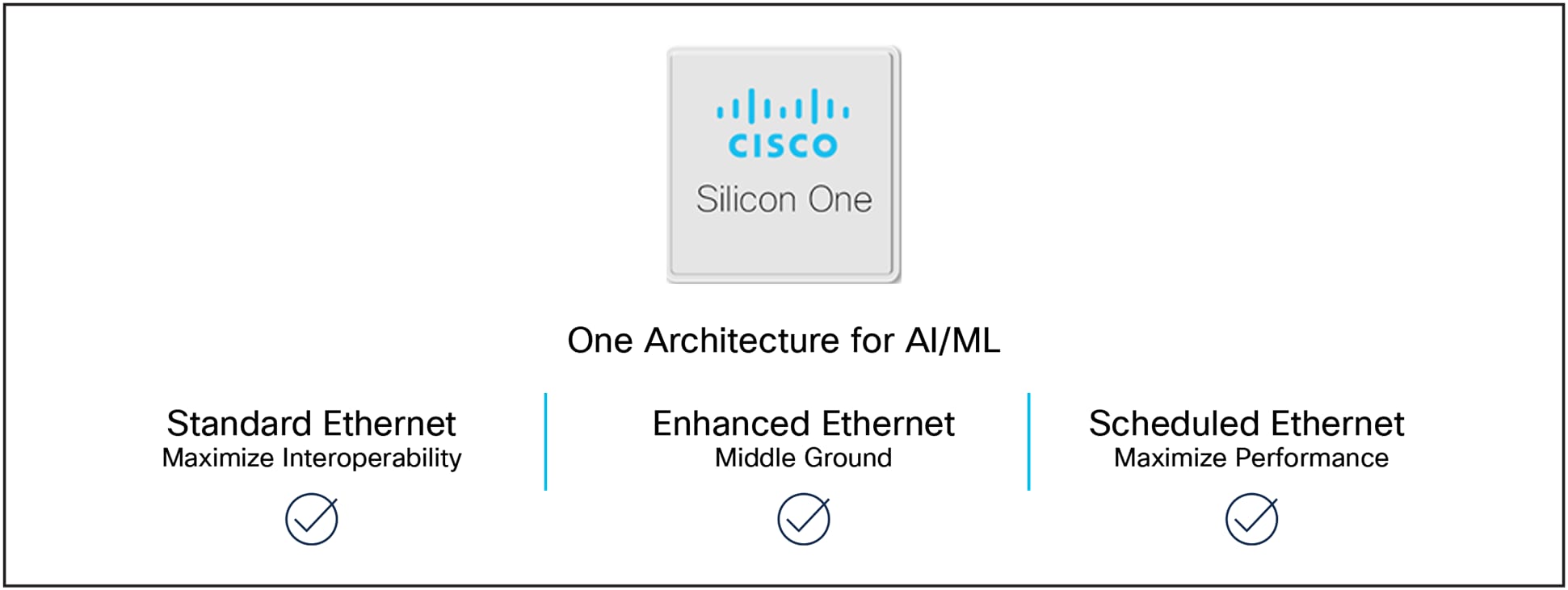
The web scale network as we know it is undergoing a massive transformation to deal with the rise of Artificial Intelligence (AI) and Machine Learning (ML). The tools that we’ve used in the past no longer suffice for the new challenge. As an industry, we must evolve our thinking and build a scalable and sustainable network for AI/ML. Standard Ethernet and Enhanced Ethernet enable fully open standards, broad availability, and favorable cost-bandwidth dynamics. Scheduled Ethernet provide ultimate non-blocking performance, but have a narrower ecosystem.
Cisco Silicon One is uniquely positioned to help web scale providers meet this challenge and allows our customers to choose via software between Standard Ethernet and Scheduled Ethernet.
Front end and back end networks
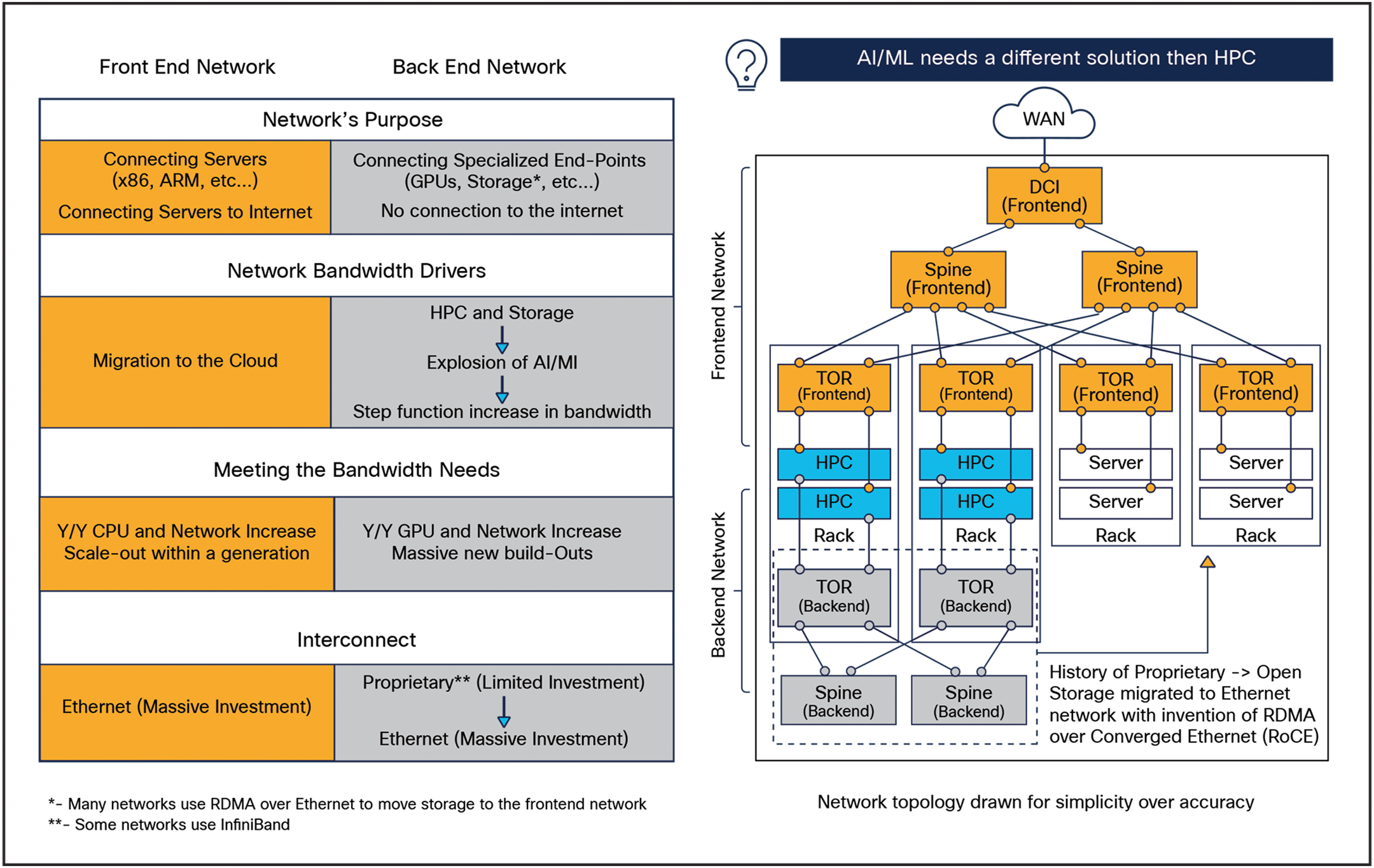
When we typically think of web scale networks, we tend to focus on what is called the front end network. This network is designed to connect generic x86 or ARM servers to one another and to the outside world. The network is typically built with Top-of-Rack (TOR) switches and multiple servers co-located in a rack. The TORs are interconnected in a CLOS topology to the spine switches. Also hanging off the spine switches are the Data Center Interconnect (DCI) routers that connect the data center to the outside world, as shown in orange in Figure 1.
Standard Ethernet is used to connect everything together in the front end network. As an open standard backed by a massive investment, the rate of innovation and the cost per gigabit of Standard Ethernet is unmatched in the industry. Many technologies have competed against Standard Ethernet, like SONET and ATM, but they are challenged to keep up with the relentless pace of bandwidth that doubles every 18-24 months.
The network that we have tended to gloss over as an industry is the back end network, shown in yellow in Figure 1. This network is designed to connect specialized endpoints to one another. Historically this network has been used for High Performance Compute (HPC) and storage applications. However, with the explosion of AI/ML workloads, web scalers are forced to build-out massive new networks to meet the demands of their customers.
The increase in AI/ML workloads is forcing a move away from the legacy, proprietary interconnects that were common in storage networks. As Ethernet has flourished, these proprietary protocols have suffered from limited investment, resulting in much higher costs per gigabit. While higher costs are never a good thing for operators, the rapid expansion of AI/ML workloads has helped force change, as the costs of legacy protocols have shifted from “suboptimal” to “intolerable.”
We’ve seen this play out before. The back end network was previously used to connect servers to storage clusters. As the storage bandwidth needs increased, the industry invented RDMA over Converged Ethernet (RoCE) and these workloads moved from the proprietary back end network to an Ethernet front end network.
The difference between front end and back end networks
The solutions that we’ve employed in the past for HPC are not good enough for the new challenges of AI/ML.
How is AI/ML different from Traditional Data Center Traffic?
To help understand why AI/ML networks are different than traditional data centers we need to understand how AI/ML works.
AI/ML clusters are generally built out of many specialized nodes, often Graphical Processing Units (GPUs), which are interconnected with a network. The algorithms that run on these GPUs are computationally intensive and perform these calculations across huge datasets, which are often larger than the memory available on a single GPU. The job is split across multiple GPUs to distribute the load, and the cluster performs an iterative set of calculations on the dataset. Each GPU performs a smaller portion of the calculation and sends the results to all its peers in a transmission process known as the All-to-All collective.
The total data transmitted by a GPU is called the collective size. This data is equally divided between all of the GPU’s peers. If a GPU was part of a 256 GPU cluster with a collective size of 1,024MB, it would transmit 1,024MB / 255 = 4MB to each other GPU. These 4MB transfers are the flow size and are multiplexed together on the network interface.
After transmission, a barrier operation occurs, which in essence stalls all of the GPUs waiting for all of the data to be received. This general process is shown in Figure 2.

Synchronization effect in the All-to-All collective causes GPUs to stall
This barrier operation makes the whole process extremely sensitive to the performance of the network. If even one slow path exists in the network, all of the GPUs will stall waiting for that one transmission to complete. This is known as the tail-latency of the job. The time it takes from the beginning of transmission to all GPUs receiving their results is the Job Completion Time (JCT). The JCT is used as a critical measure of AI performance.
One suboptimal path selection will stall the entire AI/ML job.
Said more simply: the network performance is absolutely critical.
There are many more algorithms that run on these GPUs but for brevity we will focus only on this one. Now that we understand the basics of the All-to-All collective, let’s look at how this is different from traditional datacenter traffic.
In the front end network there are many applications running on servers, where each one needs to send data to many other servers. There is a wide diversity of applications, each with its own unique traffic patterns and timing. This results in a chaotic pattern of asynchronous small bandwidth flows that on average create a relatively consistent load across the network.
Conversely: AI/ML is made up of far fewer and much higher-bandwidth flows that are synchronized with the barrier operation. As you can see in Figure 3, this causes the cumulative load on the network to rise and fall sharply. Varying latency and congestion through the network will cause some GPUs receive their data sooner and then stall, waiting for the last GPU to finish. Here, one suboptimal path selection stalls the entire AI/ML job across multiple GPUs. Said more simply, network performance is absolutely critical.
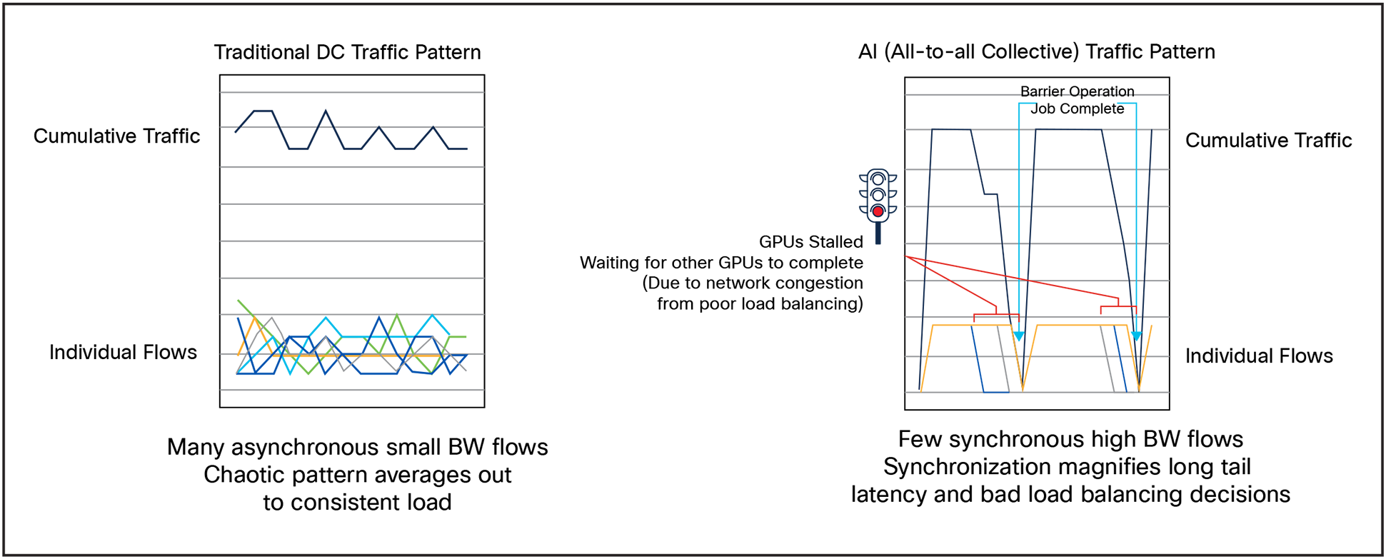
Traditional DC traffic vs. All-to-all collective
How is AI/ML different from HPC?
HPC was designed to run a single job on a large, disaggregated computer. One example that comes to mind is using HPC to calculate weather patterns due to global warming. All the nodes of the computer work together on a single large job.
Web scale AI/ML clusters are totally different.
Tools for HPC don’t scale to AI/ML applications.
These clusters are designed to run many concurrent and independent jobs over the same network. As more jobs execute independently, the job-to-job interference increases. As network congestion increases, tail latency increases. This is a normal but unfortunate event in traditional networking, but in AI/ML networks the synchronization component makes the impact of such tail latency dramatically greater.
One way to conceptualize this is to think back to the days of single threaded, single core CPUs. These machines ran a single job very well, but to run many jobs, the underlying CPU architecture needed to evolve to support multiple threads and multiple cores—all running efficiently over the same hardware. In the same way, legacy HPC networks perform well with a single job, but struggle with multiple jobs. Said more simply, tools for HPC don’t scale to AI/ML applications.
The rising importance of the network
The network has always been an important part of data centers, but in practice, the applications running on CPUs tend to be the bottleneck, hiding some of the inefficiencies of the network.
In fact, this limitation of instructions per second or instructions per watt has led to deploying smarter Ethernet Network Interface Cards (NICs) to offload functionality from general-purpose compute environments. In effect, the front end network is often compute-bound rather than network-bound. In HPC environments, the GPUs provide significantly more performance than generic servers, so HPC is both compute- and network-bound. The synchronous nature of AI/ML algorithms magnifies the effects of tail latency. Consequently, as shown in Figure 4, AI/ML is mostly network-bound.
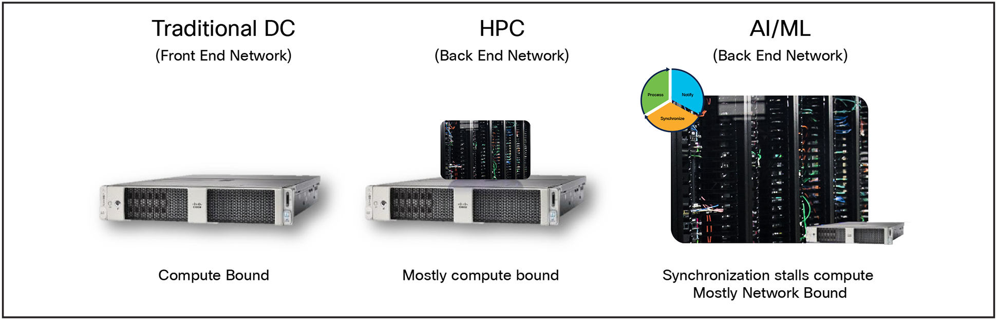
The limiting factor for network types
Load balancing options overview
Because AI/ML is network-bound, it is important to understand the options for steering traffic through the network. We consider three different options that provide good, better, and best performance.
● Good Performance: Standard Ethernet using stateless flow placement with Equal Cost Multi-Path (ECMP) hashing.
● Better Performance: Enhanced Ethernet uses stateful processing to move flows to less congested links.
● Best Performance: Scheduled Ethernet sprays packets across all available links and re-orders the packets within a flow at the egress of the network.
For more details on each of these options, please see Figure 5 below.

Load Balancing Options
Let’s look at these three options in more detail.
Load balancing – Standard Ethernet with ECMP
To understand how ECMP works and how it causes network congestion, let’s look at a simple example.
Consider the network topology shown in Figure 6, where there are three flows: blue, green and orange. Each flow arrives to a non-oversubscribed network on a dedicated input port and leaves on a dedicated output port. This is considered a non-blocking, or admissible traffic pattern. Each flow should be able to pass through the network at full rate without interference. If congestion occurs, it stems from bad network steering decisions, not the traffic pattern itself.
Non-blocking traffic pattern
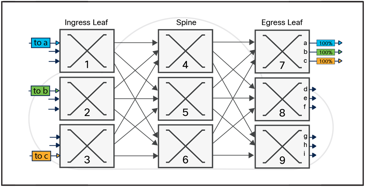
In Figure 7 we will trace these flows through a CLOS network made up of multiple ingress leafs, spines, and egress leafs, and show how the network can cause congestion even when the traffic pattern is admissible. It is drawn in what is referred to as an unfolded CLOS: the input leaf switch is shown on the left and the egress leaf switch on the right.
ECMP load balancing basics
The blue flow is from ingress leaf (1) to output port (a) on egress leaf (7). As a packet arrives at ingress leaf (1), the packet data is parsed to extract the relevant fields for forwarding the packet. The destination of the packet (Dest IP) is looked up to identify which ports could be used to reach egress leaf (7). There are three eligible paths: the packet could be sent to spine (4, 5, or 6).
In almost all cases, the order of packets within a flow must be maintained as they flow through a network.
Out-of-order delivery of TCP packets can cause data to be retransmitted, increasing network load and latency. Most other applications are similarly sensitive to packet ordering.
To guarantee in-order delivery, packets of the same flow must flow through the same path in the network. ECMP accomplishes this by hashing fields of a packet to define the flow and select a constant output port for all packets of the same flow.
Because the hash is deterministic, each packet can be hashed independently and packets from the same flow will follow the same path through the network. This enables an ECMP switch to be completely stateless, significantly simplifying the switch.
In this example, the result of the hash points to spine (4). Once the packet is received by the spine, the same functions are performed, but this time there is only a single path to reach egress leaf (7). As the packets arrive of egress leaf (7), the destination of the packet is looked up again and the packet is routed to the directly connected port (a).
Looking at the green flow destined to port (b), the same methodology is applied, however in this example the hash done on ingress leaf (2) results in the packet being sent to spine (5), and eventually to egress leaf (7) and output port (b).
As of now, the network is performing perfectly, and we can deliver both the blue and green flow through the network without congestion. But if we picture a network where thousands or even millions of flows are being hashed through the network, it’s not hard to imagine that in some conditions the result of the ECMP hash will steer packets towards congestion, causing the network to drop packets or generate Priority Flow Control (PFC) backpressure.
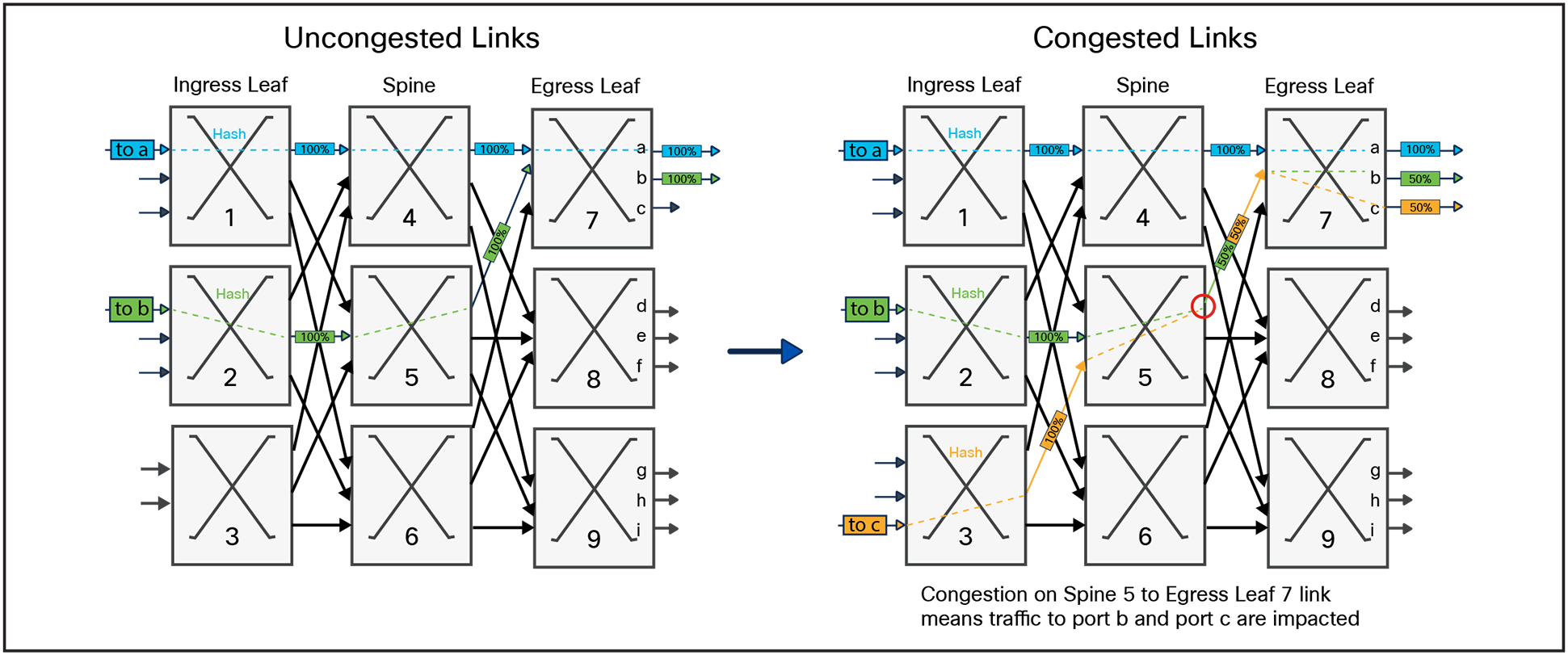
Looking at the right side of Figure 7 we can see that when the new orange flow is added it causes congestion, impacting both the green and the orange flows. To understand why this happens, let’s look through the progression of the flow step by step. When the packet arrives on ingress leaf (3), it performs ECMP which results in sending the packet to spine (5). When the packets arrive on spine (5) the green and orange flow both need to go out the link connected to leaf (7) creating a 2:1 oversubscription.
If the hash result from ingress leaf (3) selected the link towards spine (6), no congestion would have been seen. This is why the performance of an ECMP-hashed Ethernet fabric is dependent on the specific traffic characteristics flowing through the network.
In this simple example the congestion arises between the spine and the egress leaf, but it is of course possible for congestion to occur from the ingress leaf to the spine.
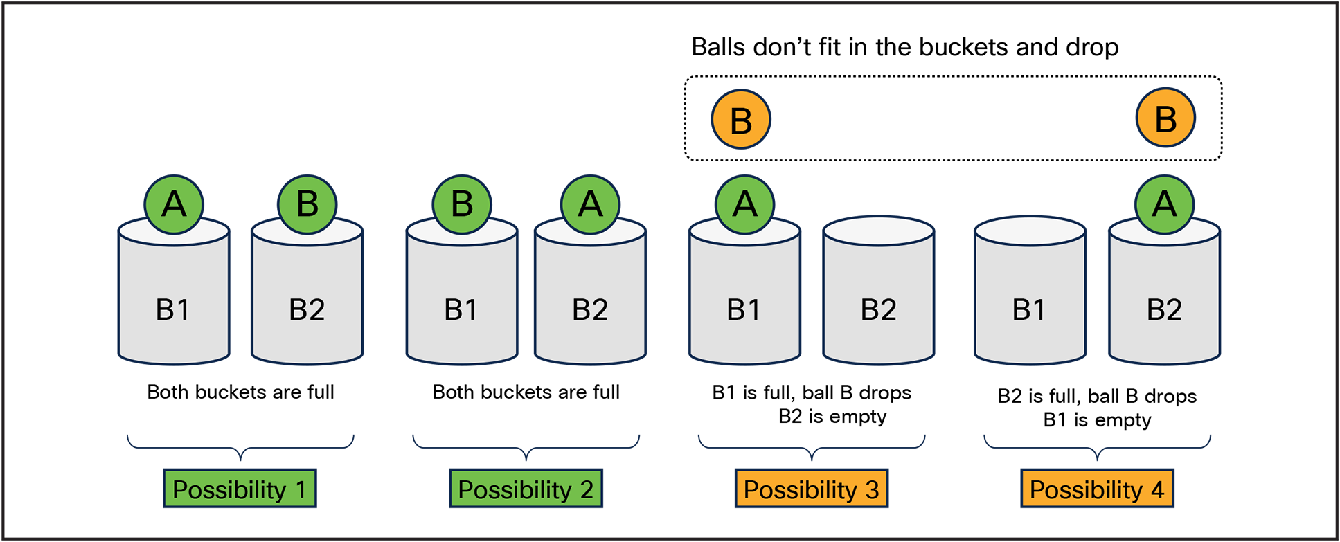
Throwing balls into bins is used frequently to explain the relationship of flows (balls), ports (bins) and oversubscription (the bin is full, the ball drops). Imagine you have two bins, and each bin can hold one ball. If you toss the two balls towards the bins, one of four things can happen, as shown in Figure 8. Two out of the four possibilities have one ball per bin. The other two outcomes overflow the bin.
Converting this example back into networking it means that we have two ports (buckets), with two flows (balls), where each flow is the full BW of the port (the size of the ball is the size of the bucket). We have a 50% probability to drop 50% of the traffic.
Buckets and balls representing ECMP Hashing (full BW, large Flows)
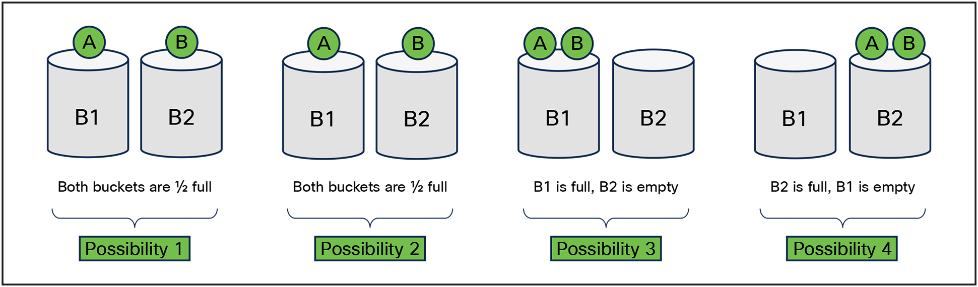
Let’s look at an example of smaller flows. Assume that we still have two ports (buckets), with two smaller flows (small balls), where each flow is ½ the BW of the port — the results are quite different. Using ECMP hash to select the port we can see that in all cases we don’t drop any traffic.
Buckets and balls representing ECMP Hashing (network overspeed, small flows)
Going into more complex examples is beyond the scope of this paper, but as we work through the examples the following important relationships appear:
● The more overspeed you have in the network, the less likely you are to drop packets.
● The smaller the flows, the less likely you are to drop packets.
● The larger the flows, the more likely you are to drop packets.
● The more flows you have (for the same bandwidth, i.e. smaller flows), the less likely you are to drop packets.
● The closer the flow size is to the port speed, the more likely you are to drop packets.
● If the flow size is bigger than the port speed, you will always drop packets.
Unfortunately, with AI/ML networks, the bandwidth demands are high in general, and the traffic is made up of high bandwidth flows. This combination makes the probability of ECMP-driven drops more likely here than in traditional front-end data center networks.
Load balancing – Enhanced Ethernet
Using telemetry to improve network performance is about making smarter load balancing decisions. If we could notify the host or the switches when there is congestion downstream, we could update the forwarding tables to avoid the congestion. To do this successfully, we must store the state communicating that a particular flow should traverse a different link.
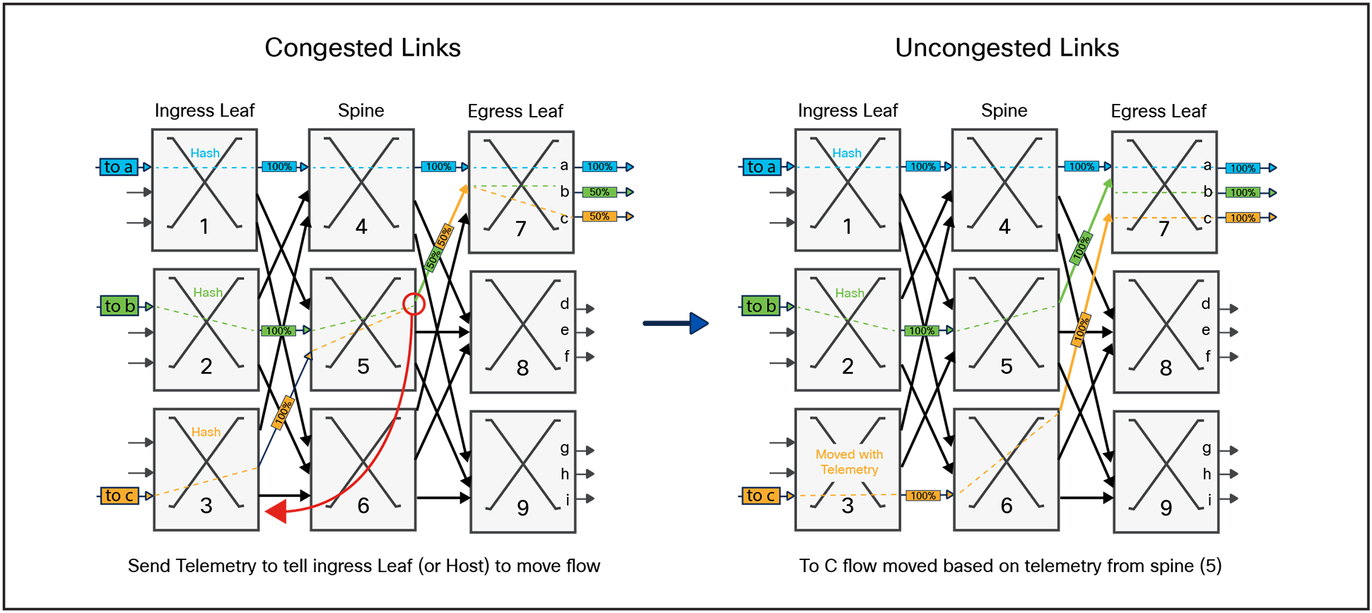
To understand how this works we will continue the example from Figure 7 above and show how telemetry can be used to rebalance the flows as shown in Figure 10.
When the orange flow destined to port (c) is sent to spine (5), the output port becomes 2:1 oversubscribed. Instead of just dropping packets, spine (5) could export information to ingress leaf (3), or the host originating the orange flow, to notify it of congestion. In this example we assume the telemetry is sent to ingress leaf (3). Based on this information it creates a new mapping for the orange flow. When ECMP is done on the orange flow the results are overwritten to point the to spine (6). Now the blue, green, and orange flows can all reach their output ports without any congestion.
This optimization requires the switches or hosts to store state information that identifies specific mappings for flows, which increases the implementation complexity. It should also be obvious that as the number of flows the switch needs to track, more state (silicon area) is required to store the state.
It’s also easy to understand that as each switch moves flows from one link to another, we have a possibility of creating a new point of congestion in the network. As the scale of the network increases, it becomes harder to converge on an uncongested state in a time- and space-efficient manner.
Working in our favor, however, is the property that AI/ML networks typically have long lasting flows rather than short ones. This reduction in churn makes it easier to converge on a stable state before the flows in the network change again.
Enhanced Ethernet
Scheduled Ethernet is a term used to describe several capabilities which, when combined, provide the ideal non-blocking performance under all traffic scenarios. To oversimplify the goal, a Scheduled Ethernet attempts to stitch together multiple switches arranged in a CLOS topology and have it mimic the behavior of a single perfect output queued switch.
To accomplish, this several technologies are used:
● Ingress Virtual Output Queues (VOQs) store packets destined to an output port and Traffic Class (TC) on the ingress leaf. There can be multiple ingress VOQs which store packets destined to an output port and traffic class.
● When there are packets enqueued for a destination, the ingress VOQ sends a request to the scheduler. The scheduler is responsible for arbitrating between all the VOQs. It divides up the available bandwidth between the requestors to enforce the Quality of Service (QoS) policy. The scheduler then sends a grant to the VOQ.
● This ensures that when a port or traffic class is oversubscribed, the packets stay in the ingress VOQ, and only packets that can be transmitted out the network will be sent from the ingress leaf, through the spine to the egress leaf.
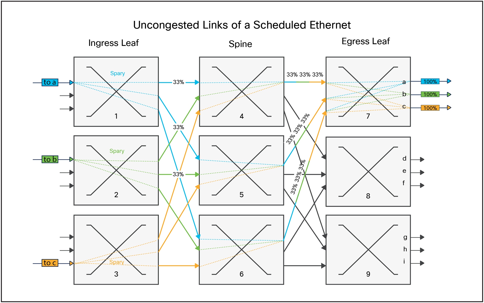
● When a packet is eligible to send from the ingress leaf, there is no hashing used to select a link. The packets are sprayed across all available links regardless of which flow the packet is associated with. If the sum of the bandwidth from the ingress leaf to the spine is equal to or greater than the bandwidth into the ingress leaf, there will never be sustained congestion.
● When packets are received at the egress leaf, the packets within a flow must be re-ordered to compensate for the variable delay across multiple paths in the network.
There are obviously many complexities that must be solved for an ingress VOQ, Scheduled Ethernet, spray and re-order fabric to be successful. But when implemented correctly, the effects on performance are dramatic.
As shown in Figure 11, as the packets move from the ingress leaf to the spine they are sprayed across all available links. Instead of a flow following one path to the egress leaf, flows take all paths to the egress leaf, thereby ensuring full utilization regardless of the specifics of the flow. Using the ball example again, the spraying effect breaks the balls into very small pieces, so you can always fit them across all the buckets every time.
Although outside the scope of this paper, there are several other benefits of this architecture.
1. Only packets which can transmit out the egress leafs ports will pass through the spine. This means that power is only consumed for “goodput” packets, saving significant power. The only place packets will be dropped is at the ingress leaf.
2. This architecture protects against incast events impacting victim flows. In a Standard Ethernet network, oversubscribed ports can consume all the bandwidth to the egress leaf, impacting traffic destined to uncongested ports. With the scheduled ingress VOQ architecture there are no victim flows.
Simply said, a Scheduled Ethernet enables the ultimate performance.
Scheduled Ethernet
Although it is easy to understand the theory behind why network performance is so important to AI/ML, it may be more impactful to specifically study the effects of various architectural choices. Here, we modeled a small example AI/ML cluster consisting of:
● 256 GPUs, each with a 200G connection to the network.
● 8 TORs, with each TOR connected to 32 GPUs within a rack.
● Four spine switches connected to the TORs in a leaf/spine CLOS topology.
● This results in a non-oversubscribed network where each TOR has 6.4Tbps of bandwidth towards the GPUs and 6.4Tbps of bandwidth towards the spines.
In our study, we ran an All-to-All Collective pattern with a collective size of 32MB, distributed evenly between all its peers in an interleaved round-robin pattern. All GPUs within a job send to all other GPUs within the job and begin transmitting simultaneously.
We then measure the Job Completion Time (JCT) to understand how the network performed. It is important to remember that the All-to-All traffic pattern is an admissible or non-oversubscribed pattern, meaning that if the network can deliver the packets correctly there should never be oversubscription. Therefore, any oversubscription that is seen is solely a result of the network flow distribution characteristics.
We studied two different traffic distribution methods.
1. Standard Ethernet with ECMP hashing.
2. A Scheduled Ethernet.
We then compared them to the perfect/theoretical ideal of raw bit transmission rate at 200G. This excludes propagation delays through the fiber as well as processing delays within the switch. It is impossible to achieve this in an actual network, but it does provide a useful baseline value for comparison purposes.
We then run several tests against this topology to study:
1. How Standard Ethernet and Scheduled Ethernet behave as we add more independent jobs to the network.
2. How Standard Ethernet performance improves as we increase the network speedup.
Effect of increasing number of simultaneous jobs
The first study we did was to analyze how the system performs as we increased the number of jobs. We began by running 256 GPUs with one job across all 256 machines up to 16 jobs each with 16 GPUs. To ensure that we are not adversely affecting the results we kept the transfer size the same at 32MB.
| # Jobs on Cluster |
Collective Size |
# Machines per Job |
# Peers |
Flow Size |
| 1 |
32MB |
256 |
255 |
32 / 255 = 0.125MB |
| 2 |
32MB |
128 |
127 |
32 / 127 = 0.251MB |
| 4 |
32MB |
64 |
63 |
32 / 63 = 0.507MB |
| 8 |
32MB |
32 |
31 |
32 / 31 = 1.03MB |
| 16 |
32MB |
16 |
15 |
32 / 15 = 2.13MB |
As shown in Figure 12, we found that both ECMP and Scheduled Ethernet performed quite well with a single job running on the cluster. ECMP took 1.24x longer than the ideal, while a Scheduled Ethernet took 1.09x longer than ideal. In comparative terms, the Scheduled Ethernet finished 1.13x quicker than Standard Ethernet.
As we increased the number of jobs the difference between ECMP and Scheduled Ethernet began to increase dramatically.
With 16 jobs ECMP is 2.11x longer than ideal, while Scheduled Ethernet remains impressively consistent with the changing patterns and is 1.11x longer than the ideal. This difference results in a Scheduled Ethernet enabling a 1.9x quicker Job Completion Time than ECMP. Importantly, the performance of a Scheduled Ethernet remains largely unaffected by the number of jobs running on the GPUs.
The performance of a Scheduled Ethernet remains largely unaffected by the number of jobs running on the GPUs.
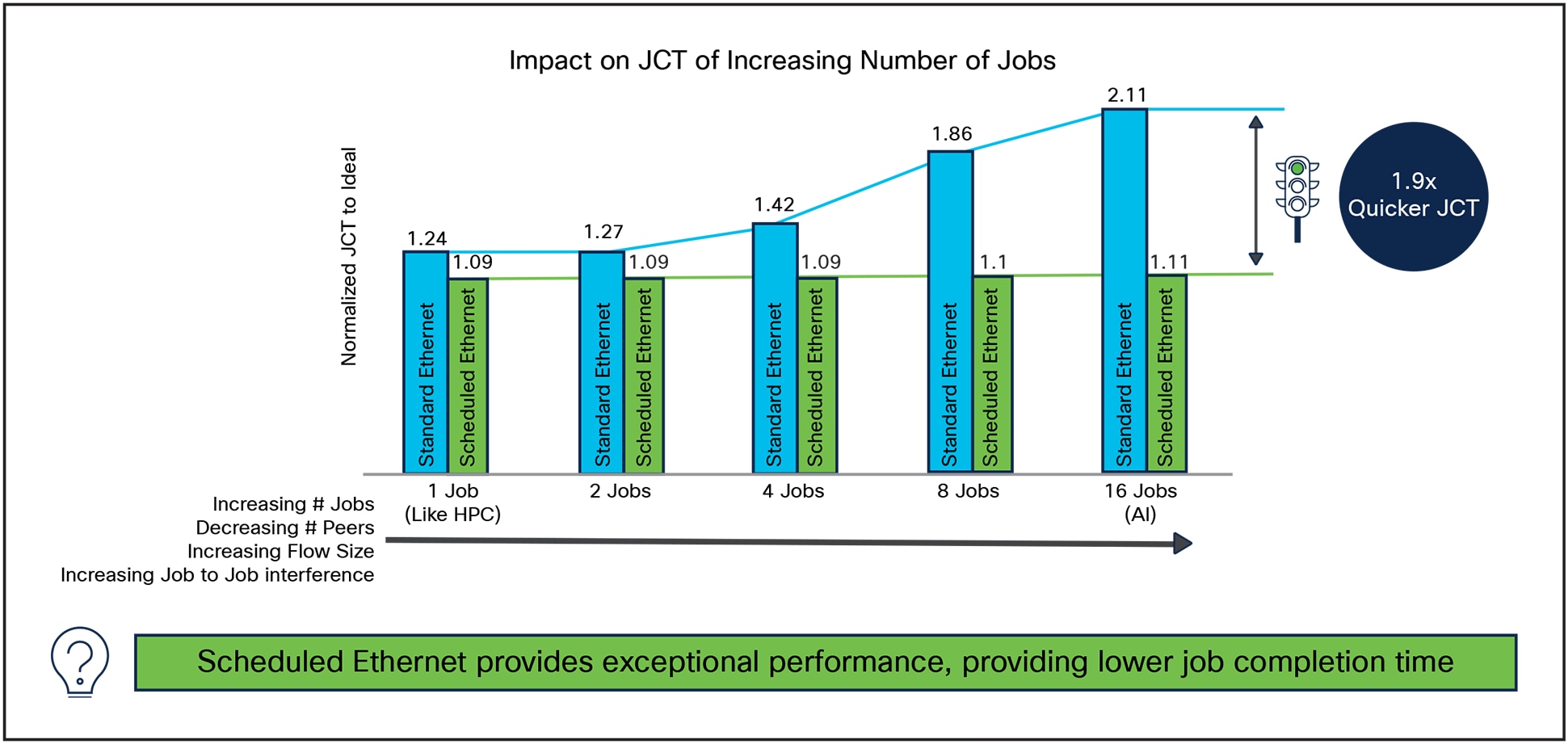
How increasing the number of jobs impacts JCT
As discussed before, it is possible to improve the performance of ECMP by using telemetry to improve load balancing decisions, however it will never reach the performance of a Scheduled Ethernet.
Adding network speedup to improve ECMP performance
We then studied how much speedup is necessary to improve the performance of Standard Ethernet ECMP with 16 jobs. We decreased the number of active GPUs under each TOR symmetrically, which has the effect of increasing the speedup across the TOR.
| # Jobs on Cluster |
Collective Size |
# Machines per Job |
Flow Size |
Active GPUs |
Speedup |
| 16 |
32MB |
16 |
2.13MB |
256 |
1x |
| 12 |
32MB |
16 |
2.13MB |
192 |
1.33x |
| 8 |
32MB |
16 |
2.13MB |
128 |
2x |
What we found is that we needed to have a network speedup of 2x to bring ECMP performance approximately in-line with a Scheduled Ethernet with a network speedup of 1x.
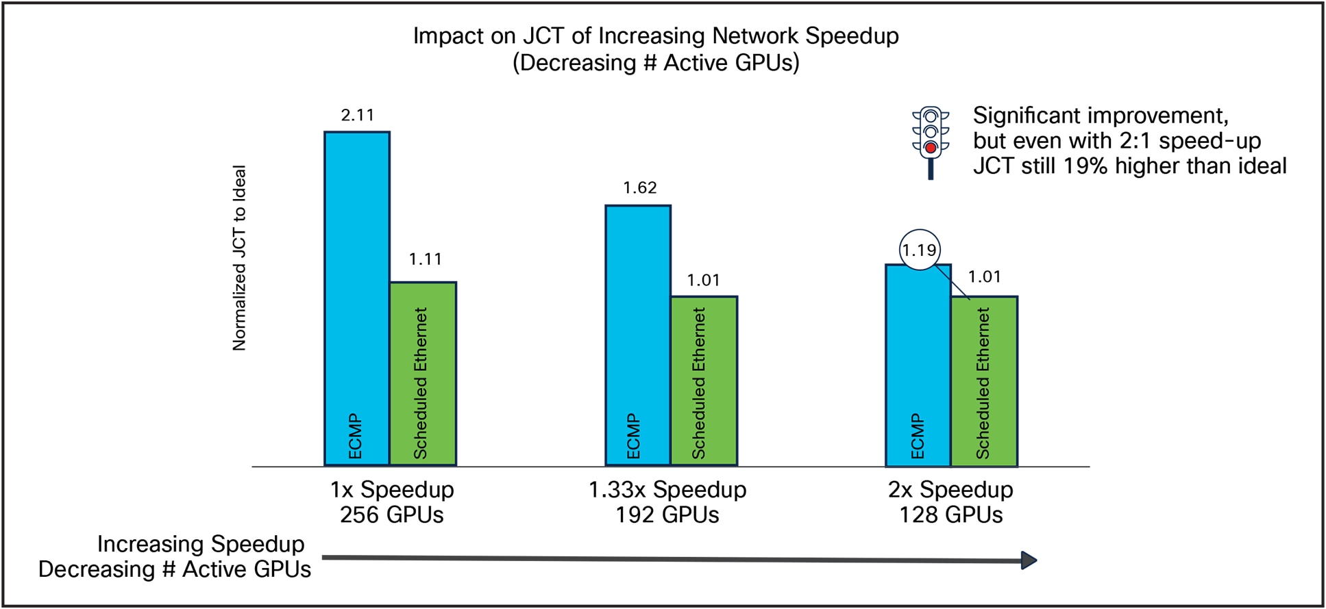
How much speedup do we need to add to Standard Ethernet to make it perform like a Scheduled Ethernet
The implication of this is significant. Looking at Figure 13, we can see that a Scheduled Ethernet with 1x speedup achieves a JCT of 1.11x above ideal, while Standard Ethernet with a 2x network speedup only achieves a JCT of 1.19x. Put another way, the Scheduled Ethernet enables over 2x the number of GPUs for the same raw bandwidth as Standard Ethernet.
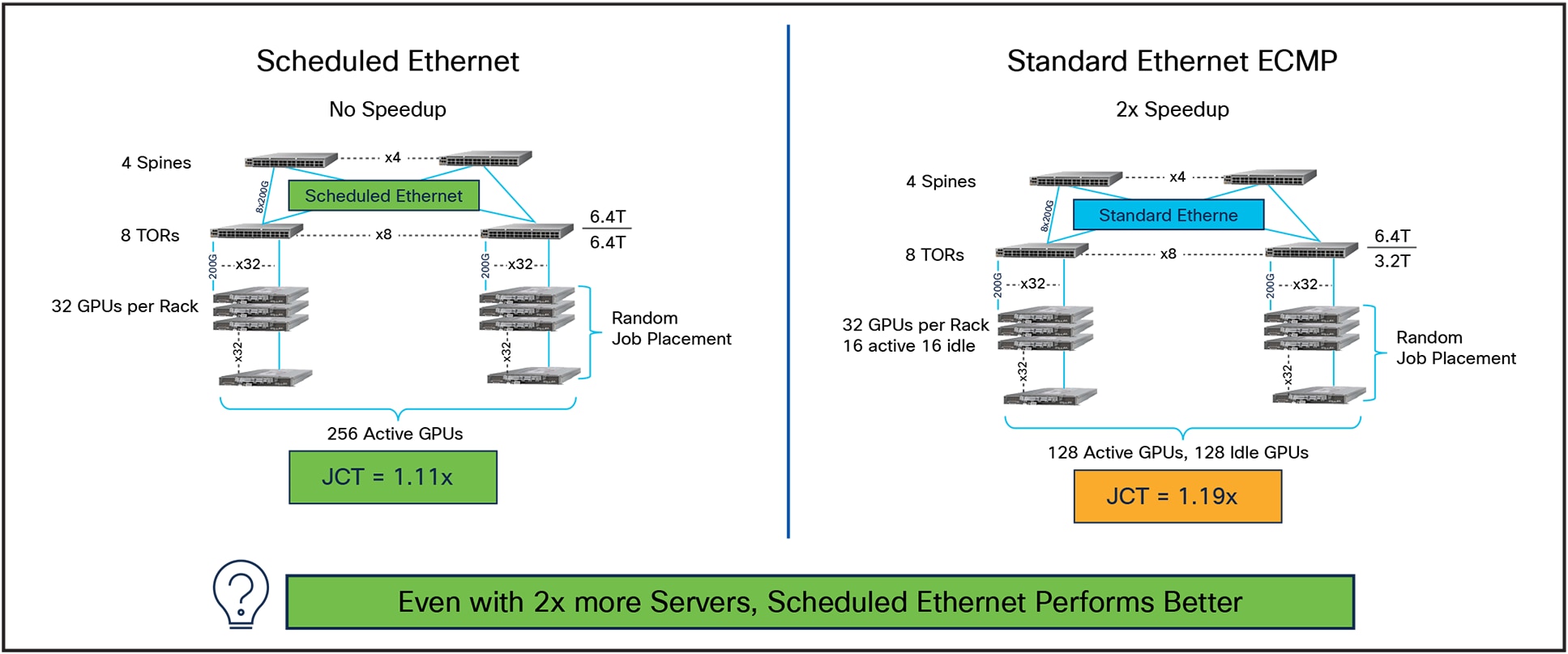
Scheduled Ethernet enables 2x more compute for the same network
We then looked closer at the results to understand why this was true. We focused on the 1.33x speedup with 192 active GPUs example. We monitored the TORs to see how often they send 802.1Qbb Priority Flow Control (PFC) XOFF messages to the GPUs. This gives us a view of how often the network is blocking the GPUs from transmitting because of network level congestion.
In Figure 15 we see a histogram shows the amount of time the GPUs receive XOFF from the network.
In blue we see:
● Six out of 192 GPUs (3%) never received flow control, meaning they were able to transmit unhindered for the entire period of the test.
● Nine out of 192 GPUs (5%) are flow controlled for 1.25mSec.
Unfortunately, because the GPUs wait for all jobs to complete, it means that 95% of the GPUs are stalled waiting for the data from 5% GPUs. The critical path here is again the tail latency. In this experiment, we have 5% of the links blocking (wasting!) 95% of the available GPU cycles.
In Figure 15 that with the Scheduled Ethernet (in green) no GPUs ever see XOFF. The Scheduled Ethernet is a 100% non-blocking network for the GPUs: there is never a point where the network slows down the GPUs.
Scheduled Ethernet is a 100% non-blocking network
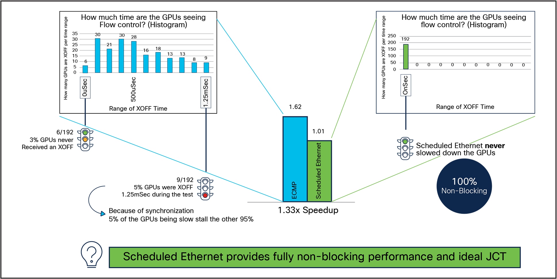
Comparing the amount of flow control from Standard Ethernet ECMP (blue) to Scheduled Ethernet (green) Flow Control
There are obviously many possible choices to build an AI/ML network from, and each of them have their own benefits.
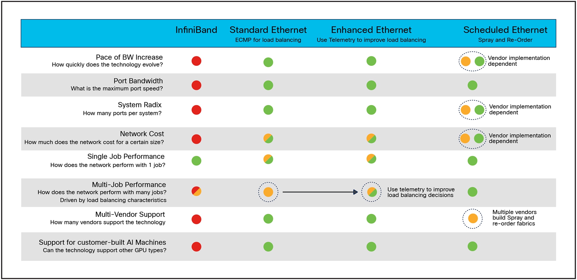
Interface Options, Pro’s and Con’s
What we see from the summary is that although there is strong performance and alignment to the HPC market with InfiniBand, the economics and multi-job performance are somewhat lacking. Importantly, as end customers build their own GPUs they likely will not have InfiniBand interfaces and therefore require a complex topology to connect into the network.
Ethernet has significant benefits in terms of the breadth of offering in the ecosystem and it performs quite well for single jobs. However, the performance constraints begin to magnify as you add additional jobs to the network. The goal of using Enhanced Ethernet is to improve multi-job performance.
Finally on the right we see a Scheduled Ethernet. There are multiple vendors who implement a Scheduled Ethernet, the cost and efficiency of the network varies by vendor. But once deployed, the performance is exceptional. Unlike Standard Ethernet these fabrics are not interoperable across vendors, so a single cluster needs to be built with a single vendor’s equipment. To mitigate this, different clusters could be built with different vendor’s equipment, thus maintaining multi-vendor support.
The Cisco Silicon One advantage
Cisco Silicon One has a unique capability in this space. Cisco Silicon One devices can be programmed via software to take on several different personalities.
1. Standalone Mode: All the serializer/de-serializer (SerDes) or ports can be configured to be Standard Ethernet. For example, our P100 device can be configured to be a true 24x800G 19.2Tbps router.
2. Linecard Mode: Approximately half of the SerDes/ports can be configured to be Standard Ethernet, and the other half can be a Scheduled Ethernet. For example, our P100 device can be configured to be 12x800G (9.6Tbps) towards Standard Ethernet, and 96x100G (9.6Tbps) towards Scheduled Ethernet.
3. Oversubscribed Linecard Mode: More than half of the SerDes/ports can be configured to be Standard Ethernet, and the rest can be Scheduled Ethernet. For example, our P100 device can be configured to be 16x800 (12.8Tbps) towards Standard Ethernet, and 64x100G (6.4Tbps) towards Scheduled Ethernet.
4. Fabric Element Mode: All the SerDes/ports can be configured to be Scheduled Ethernet. For example, our G100 can be configured to be a 256 x 100G Scheduled Ethernet element.
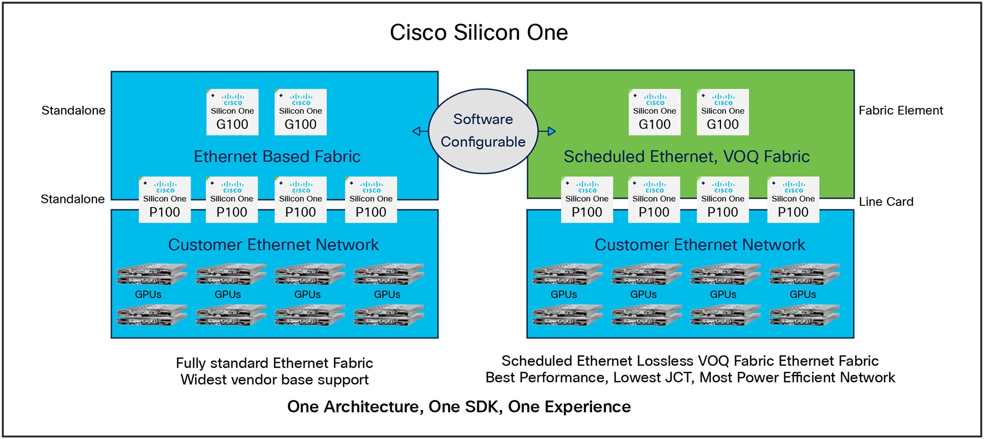
Flexibility of Cisco Silicon One
This flexibility allows you to build a CLOS network out of Silicon One devices and use software to select between Standard Ethernet, Enhanced Ethernet, of Scheduled Ethernet. This choice is not a purchase time decision; it is a choice that you can evolve over time as your needs or workloads change.
Cisco Silicon One is the only silicon architecture that allows network operators this flexibility. Using other commercially available solution requires the selection between four silicon architectures: one for InfiniBand and one for Ethernet, which may or may not be Enhanced Ethernet. A Scheduled Ethernet requires two additional silicon designs: one for the linecard elements and another for the fabric elements.
Every network operator has different concerns and priorities. Often vendors have a small set of technology to offer and so they push their solution as the best solution. This reality creates bias in most analysis.
Because Cisco Silicon One allows our customers to choose how to run our technology, we can take a fair and unbiased view of the situation and analyze the options and provide the pros and cons of each technology. This is a unique position in the industry and why we believed it was important to share our studies with network operators.
Our goal is to provide network operators with enough information to let them identify the right path forward based on their unique priorities.
Cisco Silicon One; Evolve your network
● Customers should deploy Ethernet for AI/ML networks when they want to enjoy the heavy investment, open standards, and favorable cost-bandwidth dynamics of Ethernet. They can improve the performance by investing in telemetry and minimizing network load by careful placement of AI jobs on the infrastructure.
● Customer should deploy Scheduled Ethernet for AI/ML networks when they want to enjoy the full non-blocking performance of an ingress Virtual Output Queue (VOQ), fully scheduled, spray and re-order fabric resulting in an impressive 1.9x better job completion time. Or customers who want to save cost and power by removing network elements and still achieving the same performance as Ethernet with 2x more compute for the same network.
● Watch the OCP Global Summit, October 2022 presentation.
● Watch the Cisco Knowledge Network (CKN) Webinar or download the slides
● Learn more about Cisco Silicon One.