Best Practices in Core Network Capacity Planning White Paper
Available Languages
Bias-Free Language
The documentation set for this product strives to use bias-free language. For the purposes of this documentation set, bias-free is defined as language that does not imply discrimination based on age, disability, gender, racial identity, ethnic identity, sexual orientation, socioeconomic status, and intersectionality. Exceptions may be present in the documentation due to language that is hardcoded in the user interfaces of the product software, language used based on RFP documentation, or language that is used by a referenced third-party product. Learn more about how Cisco is using Inclusive Language.
Architectural Principles of the Cisco WAN Automation Engine
Core network capacity planning is the process of ensuring that sufficient bandwidth is provisioned such that the committed core network service-level agreements can be met. The best practices described in this paper - collecting demand matrices, determining overprovisioning factors, and running simulations - are the basis of the design principles for the Cisco™ WAN Automation Engine (WAE) , especially from a planning and engineering perspective.
Capacity planning for the core network is the process of ensuring that sufficient bandwidth is provisioned such that the committed core network Service-Level Agreement (SLA) targets of delay, jitter, loss, and availability can be met. In the core network, where link bandwidths are high and traffic is highly aggregated, the SLA requirements for a traffic class can be translated into bandwidth requirements, and the problem of SLA assurance can effectively be reduced to that of bandwidth provisioning. Hence, the ability to meet SLAs is dependent on ensuring that core network bandwidth is adequately provisioned, which depends in turn on core capacity planning.
The simplest core capacity planning processes use passive measurements of core link utilization statistics and apply rules of thumb, such as upgrading links when they reach 50 percent average utilization, or some other general utilization target. The aim of such simple processes is to attempt to ensure that the core links are always significantly overprovisioned relative to the offered average load, on the assumption that this will ensure that they are also sufficiently overprovisioned relative to the peak load, that congestion will not occur, and hence that the SLA requirements will be met.
There are, however, two significant consequences of such a simple approach. First, without a networkwide understanding of the traffic demands, even an approach that upgrades links when they reach 50 percent average utilization may not be enough to ensure that the links are still sufficiently provisioned to meet committed SLA targets when network element (for example, link and node) failures occur. Second, and conversely, rule-of-thumb approaches such as this may result in more capacity being provisioned than is actually needed.
Effective core capacity planning can overcome both of these issues. Effective core capacity planning requires a way of measuring the current network load, as well as a way of determining how much bandwidth should be provisioned relative to the measured load in order to achieve the committed SLAs. Hence, in this white paper we present a holistic methodology for capacity planning of the core network that takes the core traffic demand matrix and the network topology into account. This methodology determines how much capacity the network needs in order to meet the committed SLA requirements, taking network element failures into account if necessary, while minimizing the capacity and cost associated with overprovisioning.
The methodology presented here can be applied whether Differentiated Services (DiffServ) is deployed in the core or not. Where DiffServ is not deployed, capacity planning is performed on aggregate. Where DiffServ is deployed, although the fundamental principles remain the same, capacity planning per traffic class is needed to ensure that class SLA targets are not violated.
Capacity Planning Methodology
Capacity planning involves the following steps:
1. Collect the core traffic demand matrices (either on aggregate or per class) and add traffic growth predictions to create a traffic demand forecast. This step is described in the section entitled Collecting the Traffic Demand Matrices.
2. Determine the appropriate bandwidth overprovisioning factors (either on aggregate or per class), relative to the measured demand matrices, to ensure that committed SLAs can be met. This step is described in the section entitled Determining Appropriate Overprovisioning Factors.
3. Run simulations to overlay the forecasted demands onto the network topology, taking failure cases into account if necessary, to determine the forecasted link loadings. Analyze the results, comparing the forecasted link loadings against the provisioned bandwidth and taking the calculated overprovisioning factors into account, to determine the future capacity provisioning plan required to achieve the desired SLAs. This step is described in the section entitled Simulation and Analysis.
Figure 1 illustrates this capacity planning process. The steps in the process are described in detail in the sections that follow.
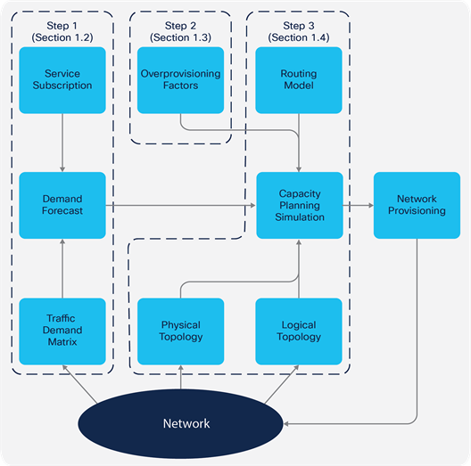
Capacity Planning Methodology
Collecting the traffic demand matrices
The core traffic demand matrix is the matrix of ingress-to-egress traffic demands across the core network. Traffic matrices can be measured or estimated to different levels of aggregation: by IP prefix, by router, by Point Of Presence (POP), or by Autonomous System (AS).
The benefit of a core traffic matrix over simple per-link statistics is that the demand matrix can be used in conjunction with an understanding of the network routing model to predict the impact that demand growth can have and to simulate “what-if” scenarios, in order to understand the impact that the failure of core network elements can have on the (aggregate or per-class) utilization of the rest of the links in the network.
With simple per-link statistics, when a link or node fails, in all but very simple topologies it may not be possible to know over which links the traffic affected by the failure will be rerouted. Core network capacity is increasingly being provisioned with the failure of single network elements taken into account. To understand traffic rerouting when an element fails, one must have a traffic matrix that aggregates traffic at the router-to-router level. If DiffServ is deployed, a core traffic matrix aggregated per Class of Service (CoS) is highly desirable.
The core traffic demand matrix can be an internal traffic matrix (that is, router to router) or an external traffic matrix (that is, router to AS), as illustrated in Figure 2, which shows the internal traffic demand matrix from one Distribution Router (DR) and the external traffic demand matrix from another.
The internal traffic matrix is useful for understanding the impact that internal network element failures will have on the traffic loading within the core. An internal matrix could also be edge to edge (for example, DR to DR) or just across the inner core (for example, Core Router [CR] to CR); a DR-to-DR matrix is preferred, as this can also be used to determine the impact of failures within a POP. The external traffic matrix provides additional context, which could be useful for managing peering connection capacity provision, and for understanding where internal network failures might affect the external traffic matrix, due to closest-exit (also known as “hot potato”) routing.
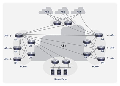
Internal and External Traffic Demands
There are a number of possible approaches for collecting the core traffic demand matrix statistics. The approaches differ in terms of their ability to provide an internal or external matrix, whether they can be applied to IP or MPLS, and whether they can provide a per-CoS traffic matrix. Further, the capabilities of network devices to provide the information required to determine the core traffic matrix can vary depending on the details of the particular vendor’s implementation.
The sections that follow discuss some of the possible approaches for determining the core traffic demand matrix.
IP flow statistics aggregation
The IP Flow Information eXport (IPFIX) protocol has been defined within the Internet Engineering Task Force (IETF) as a standard for the export of IP flow information from routers, probes, and other devices. If edge devices such as distribution routers are capable of accounting at a flow level (that is, in terms of packet and byte counts), a number of potential criteria could be used to aggregate this flow information - potentially locally on the device - to produce a traffic matrix.
When the Border Gateway Protocol (BGP) is used within an AS, for example, each router at the edge of the AS is referred to as a BGP “peer.” For each IP destination address that a peer advertises via BGP, it also advertises a BGP next-hop IP address, which is used when forwarding packets to that destination. To forward a packet to that destination, another BGP router within the AS needs to perform a recursive lookup, first looking in its BGP table to retrieve the BGP next-hop address associated with that destination address and then looking in its Interior Gateway Protocol (IGP) routing table to determine how to get to that particular BGP next-hop address. Hence, aggregating IPFIX flow statistics based on the BGP next-hop IP address used to reach a particular destination would produce an edge router to edge router traffic matrix.
When MPLS is used, a Label Switched Path (LSP) implicitly represents an aggregate traffic demand. When BGP is deployed in conjunction with label distribution by the Label Distribution Protocol (LDP), in the context of a BGP MPLS VPN service, for example, and each Provider Edge (PE) router is a BGP peer, an LSP from one PE to another implicitly represents the PE-to-PE traffic demand.
The distribution routers in the generalized network reference model we use in this paper will normally be PE routers in the context of an MPLS VPN deployment. Hence, if traffic accounting statistics are maintained per LSP, these can be retrieved, using Simple Network Management Protocol (SNMP), for example, to produce the PE-to-PE core traffic matrix.
If MPLS traffic engineering is deployed with a full mesh of Traffic Engineering (TE) tunnels, each TE tunnel LSP implicitly represents the aggregate demand of traffic from the head-end router at the source of the tunnel to the tail-end router at the tunnel destination. Hence, if traffic accounting statistics are maintained per TE tunnel LSP, these can be retrieved, using SNMP, for example, to understand the core traffic matrix.
If DiffServ-aware TE is deployed with a full mesh of TE tunnels per class of service, the same technique could be used to retrieve a per-traffic-class traffic matrix.
Demand estimation is the application of mathematical methods to measurements taken from the network, such as core link usage statistics, in order to infer the traffic demand matrix that generated those usage statistics. A number of methods have been proposed for deriving traffic matrices from link measurements and other easily measured data, and there are a number of commercially available tools that use these or similar techniques to derive the core traffic demand matrix. If link statistics are available on a per-traffic-class basis, these techniques can be applied to estimate the per-CoS traffic matrix.
Examples of demand estimation include the gravity model, tomogravity, and Cariden’s patented Demand Deduction. The accuracy and usefulness of the results depend on many factors, including how much measured traffic is available, and of what type. Demand Deduction is especially accurate in the practical cases of predicting the overall utilization after a failure, a topology change, or a metric change.[1]
Retrieving and using the statistics
Whichever approach is used to determine the core traffic matrix, the next decision to be made is how often to retrieve the measured statistics from the network. The retrieved statistics will normally be in the form of packet and byte counts, which can be used to determine the average traffic demands over the previous sampling interval. The longer the sampling interval (that is, the less frequently the statistics are retrieved), the greater the possibility that significant variation in the traffic during the sampling interval may be hidden due to the effects of averaging.
Conversely, the more frequently the statistics are retrieved, the greater the load on the system retrieving the data, the greater the load on the device being polled, and the greater the polling traffic on the network. Hence, in practice the frequency with which the statistics are retrieved is a balance that depends on the size of the network; in backbone networks it is common to collect these statistics every 5, 10, or 15 minutes.
The measured statistics can then be used to determine the traffic demand matrix during each interval. In order to make the subsequent stages of the process manageable, it may be necessary to select some traffic matrices from the collected data set. A number of possible selection criteria could be applied; one possible approach is to sum the individual (that is, router-to-router) traffic demands within each interval, and to take the interval that has the greatest total traffic demand, (that is, the peak). Alternatively, to be sensitive to outliers (for example, due to possible measurement errors), a high percentile interval such as the 95th percentile (P95) could be taken, that is, the interval for which more than 95 percent of the intervals have a lower value.
In order to be representative, the total data set should be taken over at least a week, or preferably over a month, to ensure that trends in the traffic demand matrices are captured. In the case of a small network, it might be feasible to use all measurement intervals (for example, all 288 daily measurements for 5-minute intervals), rather than to use only the peak (or percentile of peak) interval. This will give the most accurate simulation results for the network.
In geographically diverse networks, regional peaks in the traffic demand matrix may occur at a time of the day when the total traffic in the network is not at its maximum. In a global network, for example, the European region may be busy during morning office hours in Europe, while at the same time the North American region is relatively lightly loaded. It is not very easy to detect regional peaks automatically, and one alternative approach is to define administrative capacity planning network regions (for example, United States, Europe, and Asia), and apply the previously described procedure per region, to give a selected per-region traffic matrix.
Once the traffic matrix has been determined, other factors may need to be taken into account, such as anticipated traffic growth. Capacity planning will typically be performed looking sufficiently far in advance that new bandwidth can be provisioned before network loading exceeds acceptable levels. If it takes three months to provision or upgrade a new core link, for example, and capacity planning is performed monthly, the capacity planning process would need to try to predict bandwidth requirements at least four months in advance. If expected network traffic growth within the next four months was 10 percent, for example, the current traffic demand matrix would need to be multiplied by a factor of at least 1.1. Service subscription forecasts may be able to provide more granular predictions of future demand growth, possibly predicting the increase of particular traffic demands.
Determining appropriate overprovisioning factors
The derived traffic matrices described in the previous section are averages taken over the sample interval; hence, they lack information on the variation in traffic demands within each interval. There will invariably be bursts within the measurement interval that are above the average rate. If traffic bursts are sufficiently large, temporary congestion may occur, causing delay, jitter, and loss, which may result in the violation of SLA commitments even though the link is, on average, not 100 percent utilized.
To ensure that bursts above the average do not affect the SLAs, the actual bandwidth may need to be overprovisioned relative to the measured average rates. Hence, a key capacity planning consideration is to determine the amount by which bandwidth needs to be overprovisioned relative to the measured average rate, in order to meet a defined SLA target for delay, jitter, and loss. We define this as the overprovisioning factor (OP).
The overprovisioning factor required to achieve a particular SLA target depends on the arrival distribution of the traffic on the link, and the link speed. Opinions remain divided on what arrival distribution describes traffic in IP networks. One view is that traffic is self-similar, which means that it is bursty on many or all timescales (that is, regardless of the time period the traffic is measured over, the variation in the average rate of the traffic stream is the same). An alternative view is that IP traffic arrivals follow a Poisson (or more generally Markovian) arrival process. For Poisson distributed traffic, the longer the time period over which the traffic stream is measured, the less variation there is in the average rate of the traffic stream. Conversely, the shorter the time interval over which the stream is measured, the greater the visibility of burst or the burstiness of the traffic stream. The differences in the resulting measured average utilization between self-similar and Poisson traffic, when measured over different timescales, are shown in Figure 3.
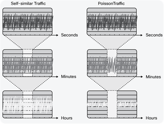
Self-Similar Versus Poisson Traffic
For Poisson traffic, queuing theory shows that as link speeds increase and traffic is more highly aggregated, queuing delays reduce for a given level of utilization. For self-similar traffic, however, if the traffic is truly bursty at all timescales, the queuing delay would not decrease with increased traffic aggregation. However, while views on whether IP network traffic tends toward self-similar or Poisson are still split, this does not fundamentally affect the capacity planning methodology we are describing. Rather, the impact of these observations is that, for high-speed links, the overprovisioning factor required to achieve a specified SLA target would need to be significantly greater for self-similar traffic than for Poisson traffic.
Note: A number of studies, both theoretical and empirical, have sought to quantify the bandwidth provisioning required to achieve a particular target for delay, jitter, and loss, although none of these studies has yet been accepted as definitive. In the rest of this section, by way of example, we use the results attained in the study by Telkamp to illustrate the capacity planning methodology. We chose these results because they probably represent the most widely used guidance with respect to core network overprovisioning.
To determine the overprovisioning factors required to achieve various SLA targets, researchers captured a number of sets of packet-level measurements from an operational IP backbone carrying Internet and VPN traffic. The traces were used in simulation to determine the bursting and queuing of traffic at small timescales over this interval, as a means of identifying the relationship between measures of link utilization that can be easily obtained with capacity planning techniques (for example, 5-minute average utilizations) and queuing delays experienced in much smaller timeframes. By using traces of actual traffic, they avoided the need to make assumptions about the nature of the traffic distribution.
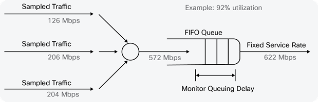
Queuing Simulation
Each set of packet measurements or “trace” contained timestamps in microseconds of the arrival time for every packet on a link, over an interval of minutes. The traces, each with a different average rate, were then used in a simulation in which multiple traces were multiplexed together and the resulting trace was run through a simulated fixed-speed queue (for example, at 622 Mbps), as shown in Figure 4.
In this example, three traces with 5-minute average rates of 126 Mbps, 206 Mbps, and 240 Mbps are multiplexed together, resulting in a trace with a 5-minute average rate of 572 Mbps, which is run through a 622-Mbps queue (that is, at a 5-minute average utilization of 92 percent). The queue depth was monitored during the simulation to determine how much queuing delay occurred. This process was then repeated with different mixes of traffic; because each mix had a different average utilization, multiple data points were produced for a specific interface speed.
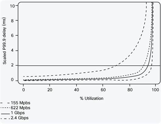
After performing this process for multiple interface speeds, the researchers derived results showing the relationship between average link utilization and the probability of queuing delay. The graph in Figure 5 uses the results of this study to show the relationship between the measured 5-minute average link utilization and queuing delay for a number of link speeds. The delay value shown is the P99.9 delay, meaning that 999 out of 1000 packets will have a delay caused by queuing that is lower than this value.
The x-axis in Figure 5 represents the 5-minute average link utilization; the y-axis represents the P99.9 delay. The lines show fitted functions to the simulation results for various link speeds, from 155 Mbps to 2.5 Gbps. Note that other relationships would result if the measured utilization was averaged over longer time periods (such as 10 minutes or 15 minutes), as in these cases there may be greater variations that are hidden by averaging, and hence lower average utilizations would be needed to achieve the same delay.
Queuing Simulation Results
The results in Figure 5 show that for the same relative levels of utilization, shorter delays are experienced for 1-Gbps links than for 622-Mbps links; that is, the level of overprovisioning required to achieve a particular delay target reduces as link bandwidth increases, which is indicative of Poisson traffic.
Taking these results as an example, we can determine the overprovisioning factor that is required to achieve particular SLA objectives. For example, if we assume that DiffServ is not deployed in the core network, and we want to achieve a target P99.9 queuing delay of 2 ms on a 155-Mbps link, then using Figure 5, we can determine that the 5-minute average link utilization should not be higher than approximately 70 percent or 109 Mbps (that is, an OP of 1/0.7 = 1.42 is required), meaning that the provisioned link bandwidth should be at least 1.42 times the 5-minute average link utilization. To achieve the same objective for a 1-Gbps link, the 5-minute average utilization should be no more than 96 percent or 960 Mbps (OP = 1.04).
Table 1. P99.9 Delay Multiplication Factors
| Number of Hops |
Delay Multiplication Factor |
| 1 |
1.0 |
| 2 |
1.7 |
| 3 |
1.9 |
| 4 |
2.2 |
| 5 |
2.5 |
| 6 |
2.8 |
| 7 |
3.0 |
| 8 |
3.3 |
Although the study by Telkamp did not focus on voice traffic, in similar studies by the same authors for Voice over IP (VoIP)-only traffic (with silence suppression), the OP factors required to achieve the same delay targets were similar. We can apply the same principle on a per-class basis when DiffServ is deployed. To assure a P99.9 queuing delay of 1 ms for a class serviced with an Assured Forwarding (AF) Per-Hop Behavior (PHB), providing a minimum bandwidth assurance of 622 Mbps (that is, 25 percent of a 2.5-Gbps link), the 5-minute average utilization for the class should not be higher than approximately 85 percent, or 529 Mbps.
Considering another example, to ensure a P99.9 queuing delay of 500 microseconds for a class serviced with an Expedited Forwarding (EF) PHB implemented with a strict priority queue on a 2.5-Gbps link, as the scheduler servicing rate of the strict priority queue is 2.5 Gbps, the 5-minute average utilization for the class should not be higher than approximately 92 percent, or 2.3 Gbps (OP = 1.09) of the link rate. Note that these results are for queuing delay only and exclude the possible delay impact on EF traffic due to the scheduler and the interface First In, First Out (FIFO) behavior.
The delay that has been discussed so far is per link and not end-to-end across the core. In most cases, traffic will traverse multiple links in the network and hence will potentially be subject to queuing delays multiple times. Telkamp’s results show that the P99.9 delay was not additive over multiple hops; rather, Table 1 shows the delay “multiplication factor” experienced over a number of hops relative to the delay over a single hop.
If the delay objective across the core is known, the overprovisioning factor that needs to be maintained per link can be determined. The core delay objective is divided by the multiplication factor from Table 1 to find the per-hop delay objective. This delay can then be looked up in the graph in Figure 5 to find the maximum utilization for a specific link capacity that will meet this per-hop queuing delay objective.
Consider, for example, a network comprising 155-Mbps links with a P99.9 delay objective across the core network of 10 ms, and a maximum of 8 hops. Table 1 shows that the 8 hops cause a multiplication of the per-link number by 3.3, so the per-link objective becomes 10 ms/3.3 = 3 ms. In Figure 5, the 3-ms line intersects with the 155-Mbps utilization curve at 80 percent. So the conclusion is that the 5-minute average utilization on the 155-Mbps links in the network should not be more than approximately 80 percent, or 124 Mbps (OP = 1.25) to achieve the goal of 10-ms delay across the core.
After obtaining the demand matrix, allowing for growth, and determining the overprovisioning factors required to achieve specific SLA targets, the final step in the capacity planning process is to overlay the traffic demands onto the network topology. This requires both an understanding of the network routing model - for example, whether an IGP, such as Intermediate System to Intermediate System (IS-IS) or Open Shortest Path First (OSPF), is used or whether MPLS traffic engineering is used - and an understanding of the logical network topology (such as link metrics and routing protocol areas) in order to understand the routing through the network that demands would take and hence to correctly map the demands to the topology.
Some tools can also run failure case simulations, which consider the loading on the links in network element failures; it is common to model for single-element failures, in which an element could be a link, a node, or a Shared Risk Link Group (SRLG). SRLGs can be used to group together links that might fail simultaneously, to represent the potential failure of unprotected interfaces sharing a common line card or circuits sharing a common fiber duct, for example.
The concept of SRLGs can also be applied to more than just links, grouping links and nodes that may represent a shared risk, in order to consider what would happen to the network loading in the presence of the failure of a complete POP, for example.
The results of the simulation provide indications of the expected loading of the links in the network; this could be the aggregate loading or the per-class loading if DiffServ is deployed. The forecasted link loadings can then be compared against the provisioned link capacity, taking the calculated overprovisioning factors into account, to determine the future bandwidth provisioning plan required to achieve the desired SLAs. The capacity planner can then use this information to identify links that may be overloaded such that SLAs will be violated, or areas where more capacity is provisioned than is actually needed.
Furthermore, WAE Design offers the toolset to perform capacity planning optimization investigations. The optimization objective can be set to minimizing the overall added capacity or minimizing the cost of added ports. The accompanying set of constraints captures the intended network design principles. For example, the following constraints can be imposed:
● The maximum utilization of interfaces can be set to a threshold in accordance to the desired overprovisioning factors
● The set of failure scenarios to be considered can be defined
● Existing circuits may be upgraded with one of these options:
◦ Existing circuits may be augmented with associated port circuits
◦ Parallel circuits may be added
● New adjacencies between nodes that were not initially connected may be proposed if capacity/cost benefits are yielded (as opposed to disallowing the addition of new adjacencies by design)
Core network capacity planning has come a long way from “rule of thumb” techniques such as upgrading links whenever they exceed a specified capacity. The best practices described in this paper - collecting demand matrices, determining overprovisioning factors, and running simulations - are all built into the design of Cisco WAN Automation Engine (WAE).
[1] For more information, see Building Accurate Traffic Matrices with Demand Deduction and Traditional Methods of Building Traffic Matrices at http://www.cisco.com.