Building Accurate Traffic Matrices with Demand Deduction White Paper
Available Languages
Bias-Free Language
The documentation set for this product strives to use bias-free language. For the purposes of this documentation set, bias-free is defined as language that does not imply discrimination based on age, disability, gender, racial identity, ethnic identity, sexual orientation, socioeconomic status, and intersectionality. Exceptions may be present in the documentation due to language that is hardcoded in the user interfaces of the product software, language used based on RFP documentation, or language that is used by a referenced third-party product. Learn more about how Cisco is using Inclusive Language.
What a traffic matrix is and how Demand Deduction using Cisco WAN Automation Engine (WAE) creates reliable traffic matrices.
Demand Deduction as a proven accurate, complete, and useful traffic simulation.
This paper outlines the need for traffic matrices and describes how Demand Deduction works. Traditional approaches fall short of building accurate, complete traffic matrices.
A network’s traffic matrix is a description, measure, or estimation of the aggregated traffic flows that enter, traverse, and leave a network. As such, a traffic matrix provides a solid understanding of the nature and levels of end-to-end traffic demands on a network. Although the need for a traffic matrix is universally recognized, producing one is often a challenge. Several tools and methods provide windows into network utilization data. However, each comes with its own limitations, and the resulting network picture is incomplete and inaccurate.
Cisco Systems designed Demand Deduction, a system for traffic matrix estimations that combines network topology data with a mathematical approach to the analysis of various types of traffic statistics. Demand Deduction is included in Cisco WAN Automation Engine (WAE) and can augment network models with traffic matrices.
What Is a Traffic Matrix?
A traffic matrix is a tabulation of end-to-end traffic between ingress and egress points, which can be broken down by service class when appropriate. Traffic matrices answer critical questions about the network. For instance, for every ingress point on a network, how much traffic is going to each egress point on that network? For service providers this could mean determining how much traffic is being exchanged between peering routers on the network, or how much traffic is going from each Autonomous System (AS) to each of the neighboring ASs.
Each traffic matrix has a scope that defines its network edge, and this inherent edge is identified and quantified according to what is needed to analyze the network.
● Internal traffic matrix: This scope consists of devices that you control. You can narrow or zoom into any portion of the network. For instance, you could look at the traffic matrix strictly from the point of view of the network core or expand the analysis to include the Provider Edge (PE) routers. This internal traffic matrix does not differentiate between discrete external sources and destinations of traffic if they are similarly connected to the network. This scope greatly simplifies the analysis and is frequently all that is needed when determining the impact of changes that occur within the network core.
● External traffic matrix: This scope generally represents an AS-to-AS mesh. When the focus is on changes that occur nearer to the edges of the network, it may be necessary to expand the scope of the analysis, and therefore to distinguish between external sources and destinations of traffic. The more distinction between the external elements, the larger this matrix becomes, and the greater the complexity of the analysis. External traffic matrices are necessary for certain types of analysis, such as when examining the impact of traffic failing over or shifting between various Border Gateway Protocol (BGP) peering locations or the impact of losing an entire border router.
Why are Traffic Matrices Important?
Traffic matrices indicate why a network’s traffic distribution looks the way it looks, and more importantly, they help predict what would happen if the network were to change. The changes can be broadly categorized as changes in topology and in traffic patterns.
Changes in topology include such events as failures, Interior Gateway Protocol (IGP) metric changes, Multiprotocol Label Switching (MPLS) Label Switched Path (LSP) shifts, and the arrival of new network elements or the decommissioning of old elements. Changes in traffic patterns include modifications such as growth or contraction in certain regions of the network, the addition of new customers, the relocation of BGP peering connections, and event-based traffic bursts.
Without a proper understanding of the network’s traffic matrix, it is very difficult to predict how network traffic will respond to such changes. Simply put, to know what will happen to the traffic on a given interface when changes occur, you must know where that traffic is coming from and where it is going. If that interface goes down, for example, some traffic might move to one interface and the rest to another or to several others, based on that traffic’s points of ingress and egress.
How to create a Traffic Matrix
Central to the idea of generating a traffic matrix is the concept of traffic demand, which represents potential traffic flowing between any two edge points in the network for any given service class (if applicable). Each demand is a single entry in a traffic matrix that identifies the amount of traffic that enters the network at point A and leaves the network at point Z. For example, 140 Mbps from er1.datacenter.acme.com to bdr3.nyc.acme.com is a traffic demand. This traffic enters the network at er1.datacenter.acme.com and traverses the network along a certain path until it reaches bdr3.nyc.acme.com, whereupon it leaves the network (presumably on its way to an external AS).
To construct a traffic matrix, you must collect information about all of the traffic and how it traverses the network. There are several approaches to this, and they can be broadly categorized as direct measurement and estimation.
Direct measurement
The direct measurement approach builds a traffic matrix by mapping traffic measurements to individual demands. The theory is that tracking the total amount of traffic between any two routers on a network results in an accurate representation of the network’s traffic matrix.
Several statistics are traditionally collected and stored, the most common ones being NetFlow, RSVP LSP, Segment Routing Traffic Matrix (SR-TM), and Label Distribution Protocol (LDP) LSP statistics. In many applications, the difficulty in gathering accurate, consistent, timely, and complete measurement data has resulted in imprecise and erroneous traffic matrices. Combining these statistics into a single traffic matrix can likewise be challenging because they do not necessarily refer to the same sources and destinations or cover the same time period. Cisco offers a scalable alternative in Cisco WAN Automation Engine (WAE) that solves these problems and provides full, accurate traffic matrices with NetFlow data.
The most accurate measurement of traffic statistics is interface statistics, which are easy to capture; there are myriad ways to do so in a timely and consistent fashion. However, traffic statistics alone do not give the required information about demand (end-to-end) traffic. They provide information only about interface (point-to-point) traffic.
Estimation
Estimation methods attempt to fit an estimation of the traffic matrix to a set of measurements taken from the network. If the estimation fits well, it is a reasonable representation of the real network traffic. Although this makes perfect sense, the obvious challenge is in producing a reasonable estimate.
A variety of traditional estimation techniques exist that produce network models of varying quality. Like direct measurements, however, they have often proven insufficiently accurate for reasons such as the following.
● Reliance on a set of measurements that is often too limited
● Minimal or unsophisticated view of network topology
● Inability to scale sufficiently to encompass the complexity of real networks
To solve the industry problems of building traffic matrices, Cisco has developed a technique called Demand Deduction. Demand Deduction has been proven in live, complex networks worldwide, producing accurate, complete, and useful traffic simulations.
What problem does Demand Deduction solve?
Before learning what Demand Deduction does, it is important to understand how demands work when the traffic matrix and network topology are known. In this scenario, determining the resulting measurements on interfaces, LSPs, and other paths is straightforward. The amount of traffic passing through an interface is the sum of all traffic demands whose routes take them through that interface. The same is true for LSPs; the amount of traffic passing through an LSP is the sum of all traffic demands that ride the LSP at some point in their journey from source to destination.
If you know where and how much traffic enters and leaves the network (that is, if you know the traffic matrix), estimating traffic measurements on each interface is simple. Figure 1 illustrates this point.
| Demand |
Demand Traffic |
Network |
| ER2 - ER5 |
4.5 Mbps |
|
| ER2 - ER6 |
3 Mbps |
|
| ER3 - ER6 |
10 Mbps |
|
| ER4 - ER1 |
7 Mbps |
|
| Interface |
Calculated Interface Traffic |
|
| CR5 - CR6 |
13 Mbps |
|
| CR5 - CR4 |
4.5 Mbps |
|
| CR1 - CR2 |
3.5 Mbps |
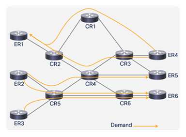
Traffic Measurements Based on Traffic Entering and Leaving the Network
Conversely, Demand Deduction starts with measured interface traffic and estimates demand traffic. More specifically, given some data regarding where traffic enters a network and where it exits, as well as various types of traffic measurements, Demand Deduction estimates a set of demands that would, if combined on this network, produce a set of measurements at or very near the observed levels. Figure 2 illustrates this point. Here the measured traffic is available for three interfaces. Demand Deduction uses this information and the topology to estimate the traffic on the edge routers. Thus, Demand Deduction determines how traffic enters, traverses, and exits the network and uses this information to produce the observed traffic measurements.
| Interface |
Measured Interface |
Network |
| CR5 - CR6 |
13 Mbps |
|
| CR5 - CR4 |
4.5 Mbps |
|
| CR1 - CR2 |
3.5 Mbps |
|
| Demand |
Estimated Demand Traffic |
|
| ER2 - ER5 |
To be calculated |
|
| ER2 - ER6 |
To be calculated |
|
| ER3 - ER6 |
To be calculated |
|
| ER4 - ER1 |
To be calculated |
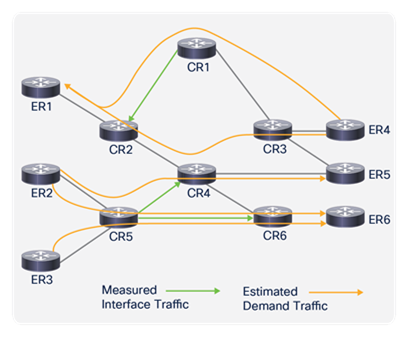
Estimating Traffic on Edge Routers Based on Observed Network Traffic
How does Demand Deduction work?
The calculations can become complex because measurements have varying levels of accuracy and completeness, and because there is usually more than one possible solution. Cisco’s Demand Deduction uses mathematical and statistical techniques to address this complexity.
The following examples represent very simple scenarios of how Demand Deduction works at the most basic level. Even inexact estimates can provide extremely accurate predictions of how traffic ultimately shifts when the network changes. However, as the amount of data and level of complexity increase, so does Demand Deduction’s ability to home in on solutions. The same principles demonstrated here apply to large networks.
The simple example in Figure 3 shows the CR1 router connected to the CR2 router with a single circuit carrying measured traffic of 10 Mbps. Traffic is flowing only left to right, from CR1 to CR2. To determine the demand traffic, first identify the ingress and egress points of network traffic and pair these into individual demands. The set of all of these pairings is called a demand mesh. This network contains only a single demand (CR1-CR2), and the demand mesh contains a single entry. Demand Deduction uses all of this information to deduce that there is only a single demand on the network, since there is a single demand on this circuit; therefore, the entirety of the traffic represented by that measurement belongs to this one demand. Thus, the CR1-CR2 demand has 10-Mbps traffic.
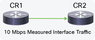
Example with Two Routers and a Single Circuit
Increasing the complexity, three edge routers and another core router are discovered (Figure 4). This network has simple connectivity of a single circuit between routers, and includes the following known information.
● The cost or metric of each circuit is 1.
● The only known measured traffic is 10 Mbps from CR1 to CR2.
● Traffic originates and terminates at the Edge Routers (ERs), and the Core Routers (CRs) carry only traffic originating from or destined for an edge router. Therefore, the demand mesh includes the following demands.
ER1 - ER2 ER2 - ER3
ER1 - ER3 ER3 - ER1
ER2 - ER1 ER3 - ER2
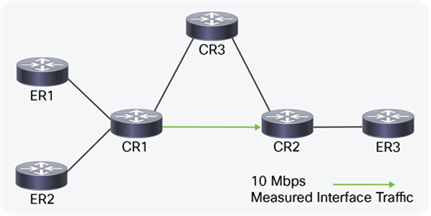
Example with Three Edge Routers and Three Core Routers
Demand Deduction uses this information to determine all edge-to-edge traffic in the demands. Since the shortest path between CR1 and CR2 is the direct circuit between them, all traffic from ER1 and ER2 destined for ER3 must use this circuit. Therefore, the demand traffic from ER1 to ER3 plus the demand traffic from ER2 to ER3 must equal 10 Mbps, and each of these demands could be anything from 0 to 10 Mbps, provided their sum is 10. Since Demand Deduction does not have enough data to determine exactly how much traffic each demand has, it balances the demands and estimates 5 Mbps for each. There is a 5-Mbps margin of error on each demand, but statistically it is likely that the real error is less than 5 Mbps.
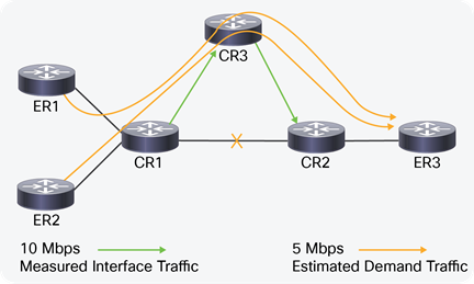
Traffic Flow when a Circuit Failure Occurs
Based on these results, Demand Deduction shows one of its greatest strengths, which is a high level of accuracy when predicting traffic shifts under failure. In the example shown in Figure 5, the circuit between CR1 and CR2 has failed. Although the demands are estimated at 5 Mbps each, there is 100 percent accuracy in predicting that 10 Mbps of traffic will shift to the alternate path via CR3 as a result of the failure. As you can see, an understanding of the traffic matrix helps you anticipate the way traffic behaves under changing network conditions. Even approximations of how the demands are divided along the network edges produce extremely accurate projections of how traffic shifts when the core network changes. This is because similar traffic near the edges tends to route similarly, shift similarly, and fail over similarly. Numerous studies have verified this behavior in practice.
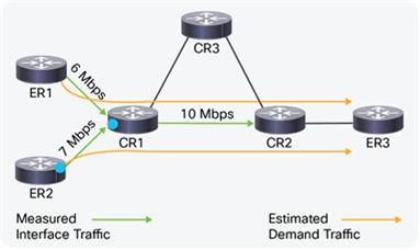
After adjustments are made to the traffic collection system, additional traffic measurements are available from the network. Including this data makes Demand Deduction results even more useful. For example, knowing that the ER1-CR1 interface traffic is 6 Mbps and the ER2-CR1 interface traffic is 7 Mbps produces a more accurate estimation of demand traffic because the possible ranges have narrower boundaries. For instance, the ER1-ER3 demand can be no less than 3 Mbps because the maximum value for the ER2-ER3 demand is the full 7 Mbps that was measured on that interface. However, the demand traffic for ER1-ER3 and ER2-ER3 must still add up to 10 Mbps. For similar reasons, the lowest value possible for the ER2-ER3 demand is 4 Mbps because the highest possible value for the ER1-ER3 demand is the full 6 Mbps that was measured on that interface.
In this scenario, Demand Deduction again balances ambiguities, essentially splitting the difference and choosing the value in the middle of the range. The resulting estimations are 4.5 Mbps for the ER1-ER3 demand and 5.5 Mbps for the ER2-ER3 demand (Figure 6). With the additional traffic measurements and narrowed range of possible demand traffic, the previous 5-Mbps margin of error is now only 1.5 Mbps.
| Interface |
Measured Interface |
Network |
| ER1 - CR1 |
6.0 Mbps |
|
| ER2 - CR1 |
7.0 Mbps |
|
| CR1 - CR2 |
10.0 Mbps |
|
| Demand |
Estimated Demand Traffic |
|
| ER1 - ER3 |
Must be 3 - 6 Mbps Estimate 4.5 Mbps |
|
| ER2 - ER3 |
Must be 4 - 7 Mbps Estimate 5.5 Mbps |
Revised Estimate of Demand Traffic
As the network increases in complexity and the possibilities multiply, the available data increases as well. In fact, the entire exercise looks more like solving a system of equations. The larger and more complex the network, the more expressions there are to solve, though the problem essentially remains the same. In effect, increasing the complexity of the network often makes solving the problem simpler.
For example, consider Figure 7, in which ER1 is dual-homed to CR1 and CR3. The topology is more complex, but solving the problem is now easier. ER2 has one shortest path to ER3. ER1 has two equal-cost paths to ER3: one via CR1 and one via CR3. Therefore, the traffic measured on the CR3-CR2 circuit must come from ER1, and it must be about 50 percent of the total traffic ER1 is sending to ER3, since the traffic is balanced evenly across both paths. With this information, Demand Deduction knows exactly what portion of the traffic on the CR1-CR2 circuit belongs to the ER1-ER3 demand, and that the remaining traffic must be coming from ER2. Also, since Demand Deduction knows how much traffic ER1 and ER2 are sending ER3, it can calculate how much traffic they are sending each other. This ability to fill in interface measurements that were not collected is critical, since measurement sets are often incomplete.
| Interface |
Measured Interface Traffic |
Network |
| ER1 - CR1 |
6.0 Mbps |
|
| ER2 - CR1 |
7.0 Mbps |
|
| CR1 - CR2 |
10.0 Mbps |
|
| CR3 - CR2 |
3.0 Mbps |
|
| Demand |
Estimated Demand Traffic |
|
| ER1 - ER3 |
3 Mbps x 2 = 6 Mbps |
|
| ER2 - ER3 |
10 Mbps - 3 Mbps = 7 Mbps |
|
| ER1 - ER2 |
6 Mbps - 3 Mbps = 3 Mbps |
|
| ER2 - ER1 |
7 Mbps - 7 Mbps = 0 Mbps |
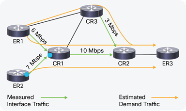
Estimate When ER1 Is Homed to Both CR1 and CR3
Regression estimates
Once Demand Deduction has combined information about the demand mesh, the network topology, and the primary source of traffic measurements (usually interface statistics) into a model that fits those measurements as closely as possible, it then considers other measurement classes to fine-tune the results. This process of adjusting the primary solution set based on additional measurement data is known as regression, and Demand Deduction can continue to refine its results by applying successive regression analyses based on a variety of secondary sources of measurement data. The more data that is available, the better the results are.
For example, assume that Demand Deduction has estimated a set of demands that results in a very close match to all network interface statistics. Further assume that some tactically deployed traffic-engineering LSPs are configured throughout the network. Demand Deduction would use the LSP traffic measurements to rebalance the estimates it has already made such that the demand estimates also result in a close fit with the LSP measurements. Once the LSP measurements have been matched as closely as possible, Demand Deduction could continue to narrow down the estimates so that access interface statistics are as closely matched as possible. Once that calculation is finished, Demand Deduction can then match NetFlow measurements as closely as possible.
Thus, rolling in additional calculations can enhance an already accurate and useful model based solely on interface statistics. While direct measurements might not be sufficient on their own, using them in combination with Demand Deduction can significantly increase the accuracy of the traffic matrix and, even more importantly, improve the accuracy of the model’s predictions near the edges of the network.
Demand Deduction using Cisco WAN Automation Engine (WAE) solves the issues with traditional practices to create accurate, complete traffic matrices. One of the capabilities that distinguish Demand Deduction is its ability to determine interface measurements that were not collected. Another is its ability to include and prioritize different traffic sources, which considerably improves the precision of the traffic matrix. Demand Deduction has been proven effective and has given service providers the ability to efficiently and accurately plan, design, engineer, and operate large, complex networks worldwide.