- About This Book
- Using the Prime Fulfillment Graphical User Interface
- Setting Up Prime Fulfillment Services
- Managing Carrier Ethernet and L2VPN Services
- Managing RAN Backhaul Services
- Managing MPLS VPN Services
- Managing MPLS Transport Profile Services
- Managing MPLS Traffic Engineering Services
- Managing Service Requests
- Managing Templates and Data Files
- Monitoring
- Performing Diagnostics
- Using the Topology Tool
- Using Inventory Manager
- Administration Tasks
- Cisco Configuration Engine Server
- Property Settings
- WatchDog Commands
- XML Reference
- Terminating an Access Ring on Two N-PEs
- Repository Views
- Inventory - Discovery
- Adding Additional Information to Services
Cisco Prime Fulfillment User Guide 6.2
Bias-Free Language
The documentation set for this product strives to use bias-free language. For the purposes of this documentation set, bias-free is defined as language that does not imply discrimination based on age, disability, gender, racial identity, ethnic identity, sexual orientation, socioeconomic status, and intersectionality. Exceptions may be present in the documentation due to language that is hardcoded in the user interfaces of the product software, language used based on RFP documentation, or language that is used by a referenced third-party product. Learn more about how Cisco is using Inclusive Language.
- Updated:
- March 20, 2015
Chapter: Using the Topology Tool
Using the Topology Tool
This chapter explains about how topology tool provides a graphical view of networks set up through the Cisco Prime Fulfillment web client. It gives a graphical representation of the various physical and logical parts of the network, both devices and links. It contains the following sections:
•![]() Accessing the Topology Tool for Prime Fulfillment-VPN Topology
Accessing the Topology Tool for Prime Fulfillment-VPN Topology
•![]() Viewing Device and Link Properties
Viewing Device and Link Properties
Introduction
The topology tool includes three types of views:
•![]() VPN view—shows connectivity between customer devices. The VPN view also gives an aggregate view of all services and individual logical and physical views of each of the services.
VPN view—shows connectivity between customer devices. The VPN view also gives an aggregate view of all services and individual logical and physical views of each of the services.
•![]() Logical view—shows logical connections set up in a selected provider region
Logical view—shows logical connections set up in a selected provider region
•![]() Physical view—displays connectivity of named physical circuits in a provider region.
Physical view—displays connectivity of named physical circuits in a provider region.
In addition, this chapter describes the following features:
•![]() Filtering and Searching—filter out unnecessary detail in large graphs or jump straight to a particular device using the search tool
Filtering and Searching—filter out unnecessary detail in large graphs or jump straight to a particular device using the search tool
•![]() Using Maps—associate maps with the individual views.
Using Maps—associate maps with the individual views.
Please note that some details, such as window decorations, are system specific and might appear differently in different environments. However, the functionality should remain consistent.
Launching Topology Tool
To launch the Topology Tool, follow these steps:
Step 1 ![]() Log into Prime Fulfillment.
Log into Prime Fulfillment.
Step 2 ![]() Choose Inventory > Logical Inventory > Topology and a window appears, as shown in Figure 12-1.
Choose Inventory > Logical Inventory > Topology and a window appears, as shown in Figure 12-1.
If you do not have the proper Java Runtime Environment (JRE) as specified at the bottom of the window, click the corresponding link for your system, follow that path, then quit the browser, log in again, and go back to the Topology Tool page.
Figure 12-1 Topology Launch Window
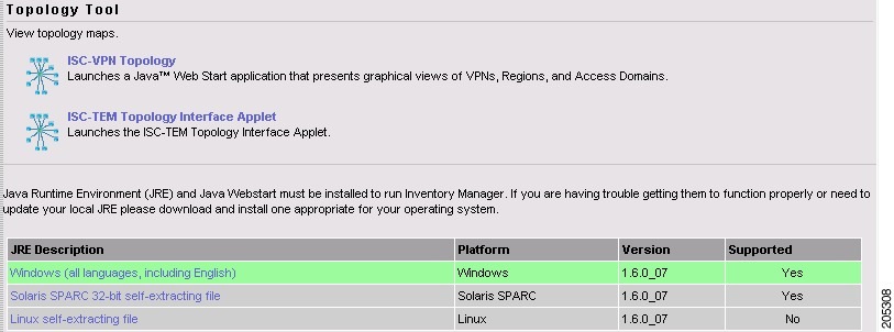
Step 3 ![]() Click Prime Fulfillment-VPN Topology in Figure 12-1, to launch the Topology Tool application on the web client.
Click Prime Fulfillment-VPN Topology in Figure 12-1, to launch the Topology Tool application on the web client.
This starts up the Java Web Start application.

Note ![]() Name resolution is required. The Prime Fulfillment HTTP server host must be in the Domain Name System (DNS) that the web client is using or the name and address of the Prime Fulfillment server must be in the client host file.
Name resolution is required. The Prime Fulfillment HTTP server host must be in the Domain Name System (DNS) that the web client is using or the name and address of the Prime Fulfillment server must be in the client host file.
Step 4 ![]() The first time Inventory Manager is activated, a Security Warning window appears. Click Start to proceed or Details to verify the security certificate, and the Desktop Integration window appears.
The first time Inventory Manager is activated, a Security Warning window appears. Click Start to proceed or Details to verify the security certificate, and the Desktop Integration window appears.
Step 5 ![]() Click Yes to integrate into your desktop environment, click No to decline, click Ask Later to be prompted the next time VPN Topology is invoked, or click Configure ... to customize the desktop integration.
Click Yes to integrate into your desktop environment, click No to decline, click Ask Later to be prompted the next time VPN Topology is invoked, or click Configure ... to customize the desktop integration.
The Login window appears whether or not a selection has been made in the Desktop Integration window.
Step 6 ![]() Enter your User Name and Password and click OK.
Enter your User Name and Password and click OK.
The Topology Tool launches and connects to the Master Prime Fulfillment server.
Conventions
Topology software uses several conventions to visually communicate information about displayed objects. The shape and color of a node representing a device depends on the role of the device, as shown in Table 12-1.

A distinct color scheme is used to highlight the link type as shown in Table 12-2:
|
|
|
|---|---|

(green) |
End-to-end wire |

(purple) |
Attachment circuit |

(brown) |
MPLS VPN link |
Finally, the four patterns shown in Table 12-3 are used to indicate the service request state:
|
|
|
|---|---|

|
Deployed, functional, pending |

|
Failed audit, invalid, broken, lost |

|
Wait deploy, requested, failed deploy |

|
Closed |
Accessing the Topology Tool for Prime Fulfillment-VPN Topology
Launch the Topology Tool as explained in Figure 12-1, "Topology Launch Window," in the "Launching Topology Tool" section and then use the following steps to access the Prime Fulfillment-VPN Topology tool.
Step 1 ![]() Choose Inventory > Logical Inventory > Topology > Prime Fulfillment-VPN Topology.
Choose Inventory > Logical Inventory > Topology > Prime Fulfillment-VPN Topology.
The Topology window shown in Figure 12-2 appears.
Figure 12-2 Topology Application Window
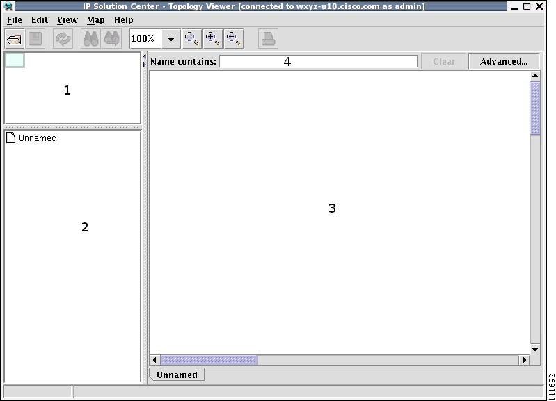
The application window is divided into four areas, as shown in Figure 12-2:
•![]() area (1)—The top left corner shows the Overview area. The colored rectangular panel, called the panner, corresponds to the area currently visible in the main area. Moving the panner around changes the part of the graph showing in the main area. This is particularly useful for large graphs.
area (1)—The top left corner shows the Overview area. The colored rectangular panel, called the panner, corresponds to the area currently visible in the main area. Moving the panner around changes the part of the graph showing in the main area. This is particularly useful for large graphs.
•![]() area (2)—The bottom left area shows the Tree View of the graph. When no graph is shown, a single node called Unnamed is displayed. When a graph is shown, a tree depicting devices and their possible interfaces and connections is displayed. The tree can be used to quickly locate a device or a connection.
area (2)—The bottom left area shows the Tree View of the graph. When no graph is shown, a single node called Unnamed is displayed. When a graph is shown, a tree depicting devices and their possible interfaces and connections is displayed. The tree can be used to quickly locate a device or a connection.
•![]() area (3)—The main area (Main View) of the window shows a graph representing connections between devices. The name of the displayed network is shown at the bottom. When no view is present, the name defaults to Unnamed.
area (3)—The main area (Main View) of the window shows a graph representing connections between devices. The name of the displayed network is shown at the bottom. When no view is present, the name defaults to Unnamed.
•![]() area (4)—Above the main window is the Filter area. It allows you to filter nodes by entering a pattern. Nodes whose name contains the entered pattern maintain the normal level of brightness. All other nodes and edges become dimmed, as shown in Figure 12-14 and the "Filtering" section.
area (4)—Above the main window is the Filter area. It allows you to filter nodes by entering a pattern. Nodes whose name contains the entered pattern maintain the normal level of brightness. All other nodes and edges become dimmed, as shown in Figure 12-14 and the "Filtering" section.
Note ![]() The bottom bar below all the areas, is a Status bar.
The bottom bar below all the areas, is a Status bar.
Views are loaded, saved, and closed using the File menu, as shown in Figure 12-3.
Figure 12-3 The File Menu
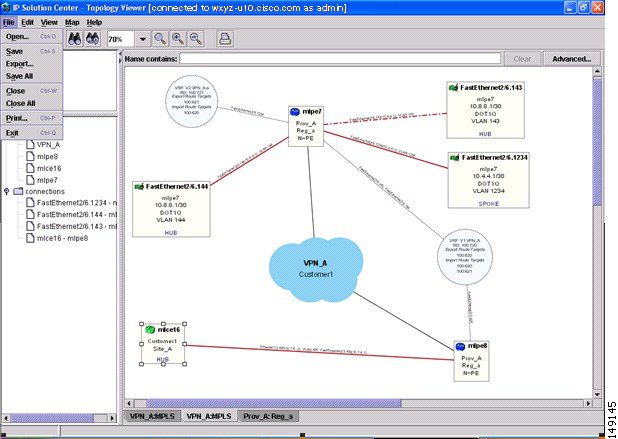
The File menu contains the following menu items:
•![]() Open—Opens a view.
Open—Opens a view.
•![]() Save—Saves the open and active view with the existing file name, if any.
Save—Saves the open and active view with the existing file name, if any.
•![]() Export—Exports the active view in either Scalable Vector Graphics (SVG), Joint Photographics Expert Group (JPG), or Portable Network Graphics (PNG) format.
Export—Exports the active view in either Scalable Vector Graphics (SVG), Joint Photographics Expert Group (JPG), or Portable Network Graphics (PNG) format.
•![]() Save All—Saves all open views.
Save All—Saves all open views.
•![]() Close—Closes the open and active view.
Close—Closes the open and active view.
•![]() Close All—Closes all open views.
Close All—Closes all open views.
•![]() Print—Prints the open and active view.
Print—Prints the open and active view.
•![]() Exit— Exits the Topology tool.
Exit— Exits the Topology tool.
Types of Views
There are three view panes in the topology application and they are described in the following sections:
•![]() VPN View, shows connectivity between devices in a VPN
VPN View, shows connectivity between devices in a VPN
•![]() Logical View, shows connectivity between PEs and CPEs in a region
Logical View, shows connectivity between PEs and CPEs in a region
•![]() Physical View, shows physical devices and links for PEs in a region.
Physical View, shows physical devices and links for PEs in a region.
The view attributes can be changed using the View menu, as shown in Figure 12-4.
Figure 12-4 The View Menu
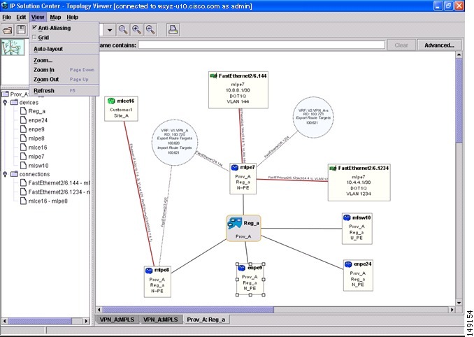
The View menu contains the following menu items:
•![]() Anti-Aliasing—When drawing a view, this creates smoother lines and a more pleasant appearance at the expense of performance.
Anti-Aliasing—When drawing a view, this creates smoother lines and a more pleasant appearance at the expense of performance.
•![]() Grid—Activates a magnetic grid. The grid has a 10 by 10 spacing and can be used to help align nodes in a view.
Grid—Activates a magnetic grid. The grid has a 10 by 10 spacing and can be used to help align nodes in a view.
•![]() Auto-Layout—Generates an automatic layout of nodes in a view. If selected, the program tries to find the most presentable arrangement of nodes.
Auto-Layout—Generates an automatic layout of nodes in a view. If selected, the program tries to find the most presentable arrangement of nodes.
•![]() Zoom—Opens a window where the desired magnification level can be specified.
Zoom—Opens a window where the desired magnification level can be specified.
•![]() Zoom In— Increases the magnification level.
Zoom In— Increases the magnification level.
•![]() Zoom Out—Decreases the magnification level.
Zoom Out—Decreases the magnification level.
•![]() Refresh—Regenerates the view. This is especially useful if the data in the repository changes. To see an updated view, select Refresh or click the Refresh toolbar button.
Refresh—Regenerates the view. This is especially useful if the data in the repository changes. To see an updated view, select Refresh or click the Refresh toolbar button.
VPN View
The VPN view shows connectivity between devices forming a given VPN. To activate the VPN view, follow these steps:
Step 1 ![]() In the menu bar, choose File > Open.
In the menu bar, choose File > Open.
or
click the Open button in the tool bar.
The Folder View window in Figure 12-5 appears displaying a directory tree with available VPNs.
Figure 12-5 Folder View Window
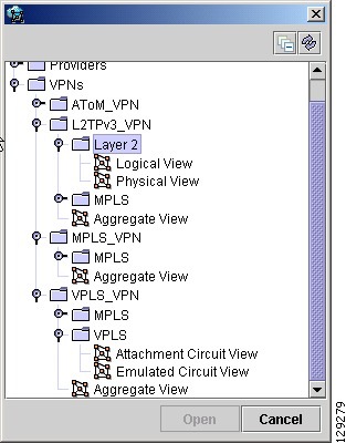
Step 2 ![]() Choose the desired VPN's folder, select the folder, and click Open.
Choose the desired VPN's folder, select the folder, and click Open.
This opens the desired folder to display any logical and physical views associated with that VPN.
Click a logical or a physical view item in the folder tree. The logical view minimizes the amount of detail and shows connectivity between customer devices. The physical view reveals more about the physical structure of the VPN. For example, for MPLS it shows connectivity between customer and provider devices and the core of the provider.
Aggregate View
The Aggregate View, as shown in Figure 12-6, shows connectivity between all customer devices, regardless of the type of technology used to connect them.
A single view might show a combination of MPLS, Layer 2, and VPLS. For MPLS, only the Customer Premises Equipment devices (CPEs) are shown.
Figure 12-6 Aggregate View
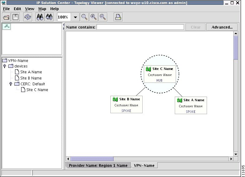
The Layer 2 VPN might in addition to CPEs show connectivity between Customer Location Edge devices (CLEs) or Provider Edge devices (PE). For VPLS, you see connectivity between CPEs. For missing CPEs, you see connectivity to PEs.
In MPLS Layer 2 VPN, the topology displays Virtual Circuit (VC) with MPLS core (as MPLS string) but with L2TPv3, the topology will display Virtual Circuit (VC) with IP core (as IP string) as shown in Figure 12-7.
Figure 12-7 Virtual Circuit with IP Core

VPLS Topology
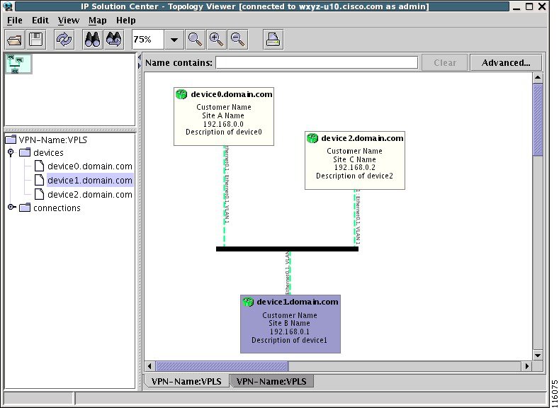
In the case of a VPLS topology, you can access an Attachment Circuit View or an Emulated Circuit View. The Attachment Circuit View corresponds to a logical view in other types of VPNs. It shows customer devices connected to a virtual private LAN, as shown in Figure 12-8.
Figure 12-8 Attachment Circuit View
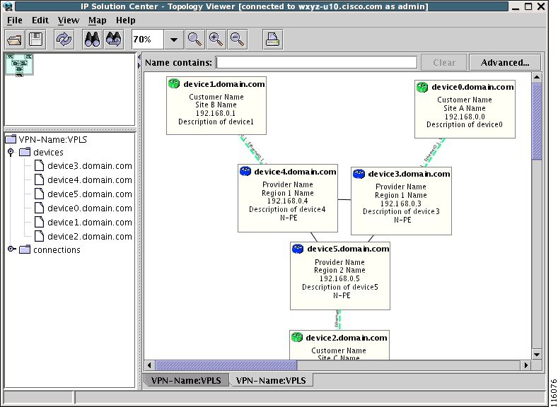
The Emulated Circuit View shows the physical connectivity details omitted in the Attachment Circuit View. It shows connectivity between provider devices and customer devices connected to provider devices, as shown in Figure 12-9.
Figure 12-9 Emulated Circuit View
Logical View
The logical view shows connectivity, created through service requests, between PEs and CPEs of a given region.
To activate the logical view, follow these steps:
Step 1 ![]() In the menu bar, choose File > Open.
In the menu bar, choose File > Open.
or
click the Open button in the tool bar.
The Folder View window, as shown in Figure 12-5, appears.
Step 2 ![]() Choose the desired VPN's folder and double-click on the desired folder.
Choose the desired VPN's folder and double-click on the desired folder.
Any logical and physical views associated with that VPN are displayed.
Step 3 ![]() To open the logical view for the selected VPN, do one of the following:
To open the logical view for the selected VPN, do one of the following:
Single-click the Logical View icon and click Open
or
Double-click the Logical View icon.
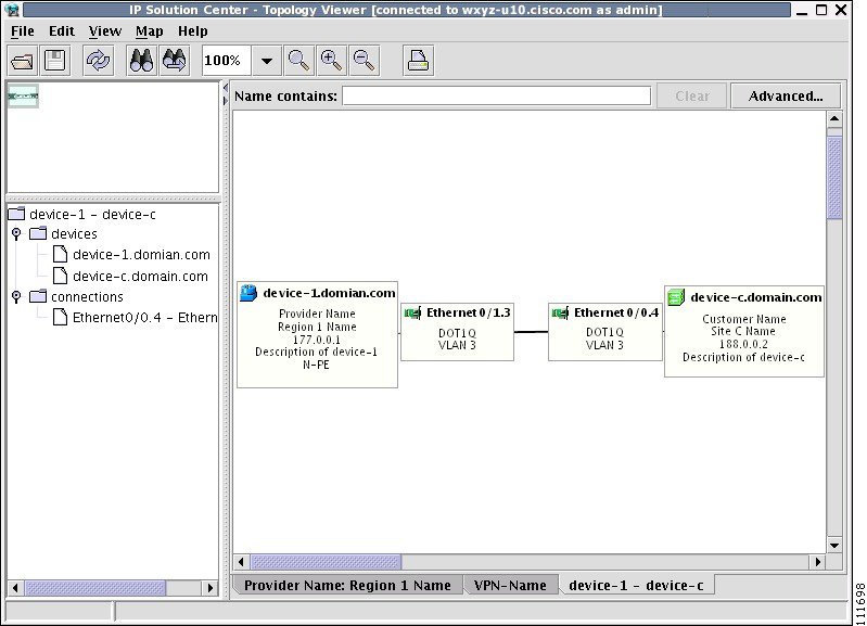
This creates a logical view for the chosen VPN, as shown in Figure 12-10.
Figure 12-10 Logical View
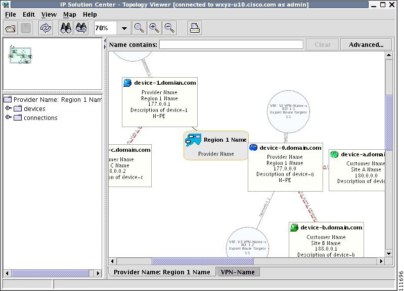
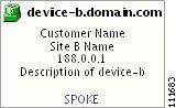
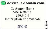
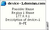
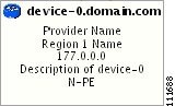
In a created view, the node, usually located in the center of the graph, is the node representing a given region of a provider. The node is annotated with the name of the region and the name of the provider.
Each node directly connected to the regional node represents a PE. The icon of a node depends on the type and the role of the device it represents (see the "Conventions" section).
Each PE is annotated with the fully-qualified device name, provider name, region name, management IP address, description, and role. A right-click on a node displays the details of the logical and physical device, interfaces, and service requests (SR) associated with the node. For the regional node, details are shown in a tabulated form.
The various node and link properties are described in detail in Viewing Device and Link Properties.
Likewise, you can right-click on a link to learn about its link properties. For example, when selecting Interfaces... for a sample serial link, a Properties window appears.
Each PE can be logically connected to one or more CPEs. Such connections are created by either MPLS VPN links or Layer 2 Logical Links. Each such connection is represented by an edge linking the given PE to a CPE. If there are more connections between a particular PE and CPE, all of them are shown. Depending on the state of a connection, the edge is drawn using a solid line (for functioning connections), dotted line (for broken connections), or dashed line (for connections yet to be established).
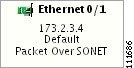
Depending on the connection type, the connection is drawn as described in Table 12-2 and Table 12-3. Each connection is annotated with the PE Interface Name (IP address), VLAN ID number, CPE Interface Name (IP address).
In the Overview area, a direct connection is drawn between a CPE and a PE, even if a number of devices are forming such a connection.
For more about viewing device properties, see Viewing Device and Link Properties.
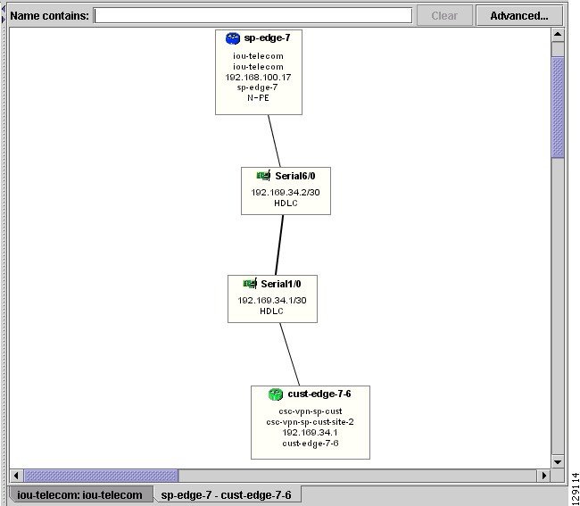
To view the details of a connection, right-click on it and select the Expand option from a pop-up menu. The expanded view, displayed in a new tab, shows all devices and interfaces making a given PE to CPE connection, as shown in Figure 12-11.
Figure 12-11 Detailed Connection View
Physical View
A physical view shows all named physical circuits defined for PEs in a given region. Each named physical circuit is represented as a sequence of connections leading from a PE through its interfaces to interfaces of CLEs or CPEs. All physical links between PEs of a given region and their CLEs or CPEs are shown. Since physical links are assumed to be in a perfect operational order, edges are always drawn with solid lines.
To activate the physical view, follow these steps:
Step 1 ![]() In the menu bar, choose File > Open.
In the menu bar, choose File > Open.
or
click the Open button in the tool bar.
The Folder View window, as shown in Figure 12-5, appears.
Step 2 ![]() Choose the desired VPN's folder and double-click on the desired folder.
Choose the desired VPN's folder and double-click on the desired folder.
Any logical and physical views associated with that VPN are displayed.
Step 3 ![]() To open the physical view for the selected VPN, do one of the following:
To open the physical view for the selected VPN, do one of the following:
Single-click the Physical View icon and click Open
or
Double-click the Physical View icon.
This creates a physical view for the chosen VPN, as shown in Figure 12-12.
Figure 12-12 Physical View
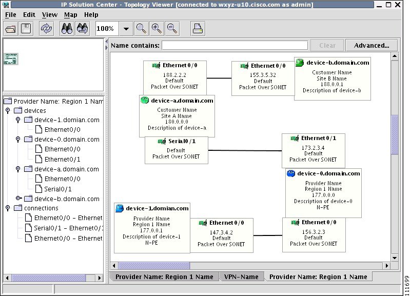
In this view, each device is connected with a thin line to the interfaces it owns. Interfaces are connected to other interfaces with thick lines. If there is more than one connection between two interfaces, they are spaced to show all of them.
The tree shows devices and connections. Each device can be a folder, holding all interfaces connected to it.
Viewing Device and Link Properties
In the logical view, you can view the properties of both devices and links. In the physical view, only properties of physical devices are accessible.
Thus, device properties can be viewed in both the logical and physical views.
Device Properties
To view the properties of a device, right-click the device. The Device Properties menu appears.
The following properties are available:
Logical Device...—View the logical properties of the device.
Physical Device...—View the physical properties of the device.
Interfaces...—View interface properties of the device.
Service Requests...—View service request properties associated with the device.
Logical Device
When right-clicking a device and selecting Logical Device..., the logical device properties window appears.
The logical properties window displays the following information:
Device Name—Name of the device.
Provider Name—Name of the provider whom the device is serving.
Region Name—Name of the provider region.
Loopback Address—IP address of the loopback address.
Role Type—Role assigned to the device.
Physical Device
When right-clicking a device and selecting Physical Device..., the physical device properties window appears.
The physical properties window displays the following information:
Name—Name of the device.
Description—User-defined description of the device.
Collection Zone—Collection zone for device data.
IP Address—IP address of the interface used in the topology.
User ID—User ID for the interface.
Enable User—Password for the interface.
Device Access Protocol—Protocol used to communicate with the device.
Config Upload/Download—Upload/download method for the configuration file.
SNMP Version—Simple Network Management Protocol (SNMP) version on the device.
Community String RO—public or private
Community String RW—public or private
SNMP Security Level—Simple Network Management Protocol (SNMP) security level.
Authentication User Name—User name for performing authentication on the device.
Authentication Algorithm—Algorithm used to perform authentication.
Encryption Algorithm—Encryption algorithm used for secure communication.
Terminal Server—Name of the terminal server.
Terminal Server Port—Port number used by the terminal server.
Platform—Hardware platform.
Software—IOS version or other management software on the device.
Image Name—Boot image for device initialization.
Serial Number—Serial number of the device.
Interfaces
When right-clicking a device and selecting Interfaces..., the interface properties window appears.
The interface properties window displays the following information:
Name—Name of the device.
IP Address—IP address of the device.
IP Address Type—STATIC or DYNAMIC.
Encapsulation—Encapsulation used on the interface traffic.
Description—Description assigned to the interface, if any.
Select (link)—If a connection is attached to the interface, a drop-down list at the bottom of the window allows you to choose between the interfaces available on the device.
Service Requests
When right-clicking a device and selecting Service Requests..., the service request (SR) properties window appears.
The service request properties window displays the following information:
Job ID—SR identifier.
Type—Protocol type used in the SR.
State—SR state.
Operation Type—Encapsulation used on the interface traffic.
Creator—Description assigned to the interface, if any.
Creation Time—Date and time when the SR was created.
Customer Name—Name of customer associated with the SR.
Last Modified—Date and time when the SR was last modified.
Description—User-defined description of the SR.
Select (SR)—If more than one SR is associated with the interface, the drop-down list at the bottom of the window allows you to choose between these SRs.
Link Properties
To view the properties of a given link, right-click the link. The Link Properties menu appears.
The following options are available:
Expand—View link details, including devices local to the link not shown in the general topology.
Service Request...—View service request properties associated with the link.
MPLS VPN—View the MPLS VPN properties of the link. Other link protocol properties than MPLS VPN are currently not available.
Expand
When right-clicking a link and selecting Expand..., the Topology Display will display any devices and connections local to that link. An Expand Link window similar to the one in Figure 12-13 will appear.
Figure 12-13 Expand Link Window
Properties information for devices and links can only be obtained in the master view as described earlier in this section.
Service Request
When right-clicking a link and selecting Service Requests..., the service request (SR) properties window appears.
The service request properties window displays the following information:
Job ID—SR identifier.
Type—Protocol type used in the SR.
State—SR state.
Operation Type—Encapsulation used on the interface traffic.
Creator—Description assigned to the interface, if any.
Creation Time—Date and time when the SR was created.
Customer Name—Name of customer associated with the SR.
Last Modified—Date and time when the SR was last modified.
Description—User-defined description of the SR.
Select (SR)—If more than one SR is associated with the interface, the drop-down list at the bottom of the window allows you to choose between these SRs.
MPLS VPN
When right-clicking a link that is configured for MPLS VPN and selecting MPLS VPN..., the MPLS VPN properties window appears.
The service request properties window displays the following information:
Status—Status of the MPLS VPN link.
Status Message—Displays any error or warning messages.
Operation Type—MPLS operation type.
Policy Type—The policy type applied to the link.
Data MTD Threshold—Memory Technology Driver (MTD) data threshold.
Default MTD Address—Default MTD IP address.
Data MTD Subnet—Data MTD subnet.
Data MTD Size—Data MTD size.
SOO Enabled—Site of Origin Enabled - Yes or No.
Manual Config—Yes or No.
Filtering and Searching
On large graphs, the amount of detail can be overwhelming. In such cases, filtering might help eliminate unnecessary details, while searching can lead to a prompt location of a device you want to examine further.
Both advanced filtering and searching use the same window to enter conditions on nodes to be either filtered or located. The filtering area also allows you to quickly filter viewed objects by name.
Filtering
The topology view can be filtered in two ways, simple and advanced.
Simple Filtering
To perform simple filtering of the view, follow these steps:
Step 1 ![]() Enter a string in area (4) of the main window, as shown in Figure 12-2.
Enter a string in area (4) of the main window, as shown in Figure 12-2.
Step 2 ![]() Press Enter to dim all objects whose name does not contain the specified string.
Press Enter to dim all objects whose name does not contain the specified string.
For example, to locate nodes that contain string router in their name you would enter router in area (4) and click Enter. All objects whose name does not contain the entered string are dimmed, as shown in Figure 12-14.
Figure 12-14 Physical View with Dimmed Nodes
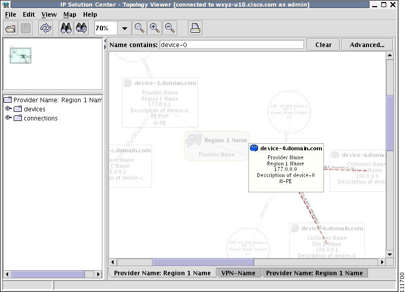
Note ![]() Regular expressions are supported but only in the advanced window (click Advanced... button). For example, by entering ^foo.*a, you only request nodes that have names starting with "foo" followed by arbitrary characters and containing the letter 'a' somewhere in the name. The regular expressions must follow the rules defined for Java regular expressions.
Regular expressions are supported but only in the advanced window (click Advanced... button). For example, by entering ^foo.*a, you only request nodes that have names starting with "foo" followed by arbitrary characters and containing the letter 'a' somewhere in the name. The regular expressions must follow the rules defined for Java regular expressions.
Advanced Filtering
To perform advanced filtering, follow these steps:
Step 1 ![]() Open the advanced filtering window by clicking the Advanced... button.
Open the advanced filtering window by clicking the Advanced... button.
The Advanced Filter window appears.
Step 2 ![]() Make the desired filtering elections.
Make the desired filtering elections.
The window allows you to enter one or more conditions on filtered nodes. The first drop-down list allows you to specify the attribute by which the filtering is performed. The second allows you to decide how the matching between the value of the attribute and text entered in the third column is performed.
The following matching modes are supported from the drop-down list:
•![]() contains—The attribute value is fetched from the device and it is selected if it contains the string given by you. The string can be located at the start, end, or middle of the attribute for the match to succeed. For example, if the pattern is cle the following values match it in the contains mode: clean, nucleus, circle.
contains—The attribute value is fetched from the device and it is selected if it contains the string given by you. The string can be located at the start, end, or middle of the attribute for the match to succeed. For example, if the pattern is cle the following values match it in the contains mode: clean, nucleus, circle.
•![]() starts with—The value of the attribute must start with the string given by you. For example, if the pattern is foot, footwork matches, but afoot does not.
starts with—The value of the attribute must start with the string given by you. For example, if the pattern is foot, footwork matches, but afoot does not.
•![]() ends with—This is the reverse of the starts with case, when a given attribute matches only if the specified pattern is at the end of the attribute value. In this mode, for example, the pattern foot matches afoot but not footwork.
ends with—This is the reverse of the starts with case, when a given attribute matches only if the specified pattern is at the end of the attribute value. In this mode, for example, the pattern foot matches afoot but not footwork.
•![]() doesn't contain—In this mode, only those strings that do not contain the given pattern match. The results are opposite to that of the contains mode. For example, if you specify cle in this mode, clean, nucleus, and circle are rejected, but foot is deemed to match, because it does not contain cle.
doesn't contain—In this mode, only those strings that do not contain the given pattern match. The results are opposite to that of the contains mode. For example, if you specify cle in this mode, clean, nucleus, and circle are rejected, but foot is deemed to match, because it does not contain cle.
•![]() matches—This is the most generic mode, in which you can specify a full or partial expression that defines which nodes you are interested in.
matches—This is the most generic mode, in which you can specify a full or partial expression that defines which nodes you are interested in.
By clicking one of the two radio buttons, Match any conditions or Match all conditions, you can request that any or all of the conditions are matched. In the first case, you can look for devices where, for example, the name contains cisco and the management IP address ends with 204. When all conditions must be met, it is possible to look for devices that, for example, have a given name and platform.
Click More or Fewer to add more rows of conditions or remove existing rows of conditions.
By default, all matches are performed without regard for upper or lower case. However, in some cases it is beneficial to have a more exact matching that takes the case into account. To do so, check the Match case check box.
Step 3 ![]() Click OK to start the filtering process. Click Cancel to hide the window without any changes to the state of the filters.
Click OK to start the filtering process. Click Cancel to hide the window without any changes to the state of the filters.
The Clear button allows you to clear all conditions. Clicking Clear followed by OK effectively removes all filtering, restoring all nodes to their default brightness level. If filtering is active, the same can be achieved by clicking Clear in area (4) of the main window, as shown in Figure 12-2.
Searching
Searching can be conducted by using the menus or the tool bar. To perform a search, follow these steps:
Step 1 ![]() Select Find in the Edit menu
Select Find in the Edit menu
or
Click the Find icon in the main toolbar.
Both approaches bring up the same window, as shown in Figure 12-15.
Again, you can enter one or more conditions to locate the node.
Figure 12-15 Find Window
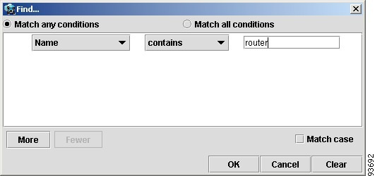
Step 2 ![]() Make the desired filtering selections.
Make the desired filtering selections.
Match modes, case check box, and the radio button are used as described under Advanced Filtering.
Step 3 ![]() Click OK to start searching for the first node that matches the given criteria.
Click OK to start searching for the first node that matches the given criteria.
If found, the node is highlighted and the view is shifted to make it appear in the currently viewed area of the main window.
Step 4 ![]() After the first search, press F3 or click the Find Again button to repeat the search
After the first search, press F3 or click the Find Again button to repeat the search
If more than one node matches the condition the Find Again function highlights each one of them. If no nodes match the entered criteria, the Object Not Found window appears.
Using Maps
You can associate a map with each view. Currently, the topology viewer only supports maps in the Environmental Systems Research Institute, Inc. (ESRI) shape format. The following sections describe how to load maps and selectively view map layers and data associated with each map.
The map features are accessed from the Map menu shown in Figure 12-16.
Figure 12-16 The Map Menu
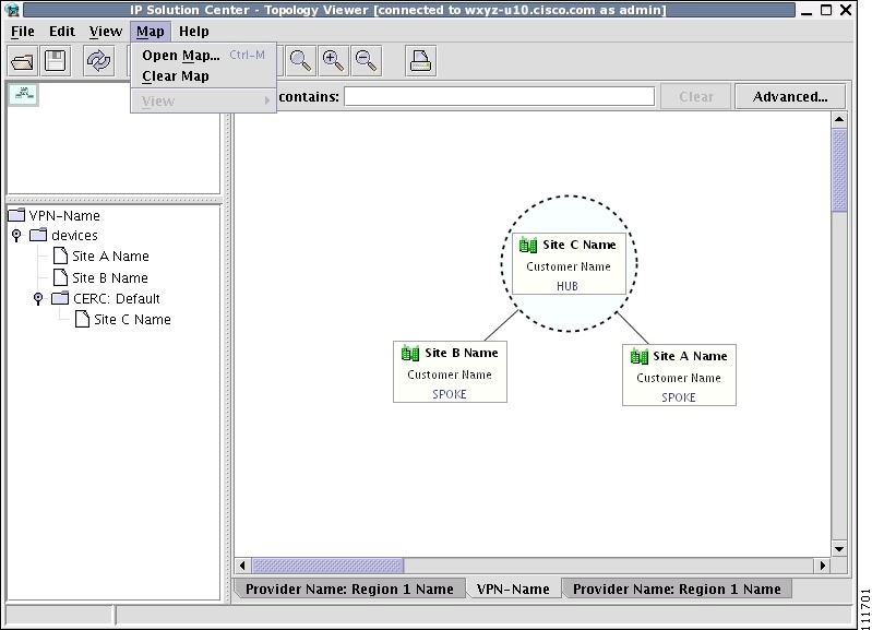
The Map menu contains the following menu items:
•![]() Open Map—Loads a map into the application
Open Map—Loads a map into the application
•![]() Clear Map—Clears the active map from the current view
Clear Map—Clears the active map from the current view
•![]() View—Allows you to select which layers in the map should be displayed (for example, country, state, city).
View—Allows you to select which layers in the map should be displayed (for example, country, state, city).
Loading a Map
You might want to set a background map showing the physical locations of the displayed devices. To load a map, follow these steps:
Step 1 ![]() In the menu bar, select Map > Open Map....
In the menu bar, select Map > Open Map....
or
Press Ctrl-M
Step 2 ![]() Make your selections in the Load Map window.
Make your selections in the Load Map window.
The right-hand side of the window contains a small control panel, which allows you to select the projection in which a map is shown. A map projection is a projection that maps a sphere onto a plane. Typical projections are Mercator, Lambert, and Stereographic.
For more information on projections, consult the Map Projections section of Eric Weisstein's World of Mathematics at:
http://mathworld.wolfram.com/topics/MapProjections.html
For each projection, you can also select the region of the map to be shown. In most cases, the predefined values should be sufficient.
If desired, make changes to the settings in the Longitude Range and Latitude Range fields.
Step 3 ![]() Select a map file and click Open to load the map.
Select a map file and click Open to load the map.
Selecting the map file and clicking the Open button starts loading it. Maps can consist of several components and thus a progress window is shown informing you which part of the map file is loaded.
Layers
Each map can contain several layers. For example most country maps have country, region, and city layers, as shown in Figure 12-17.
Figure 12-17 Map Layers
After a map is loaded, the View submenu of the Map menu is automatically populated for you. A name of each available layer is shown together with the check box indicating visibility of the layer. If a given map shows too many details, you can turn off some or all layers by unchecking the corresponding check box(es). The same submenu can be used to restore visibility of layers.
If an incorrect map is loaded or the performance of the topology tool is unsatisfactory with the map loaded, you can clear the map entirely. To do this, select Clear Map from the Map menu. Maps are automatically cleared if another map is loaded.
Consequently if you want just to load another map, there is no need to clear the existing map. The act of loading a new map does this.
Map Data
If map data files are successfully loaded with the map, the right field of the Status bar shows the longitude and latitude location of the cursor on the map. If map objects, such as cities, lakes, and so on, have data associated with them, their names are displayed after the longitude and latitude coordinates.
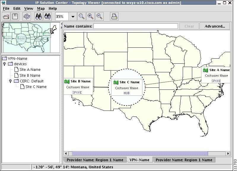
Node Locations
After a map is successfully loaded, the view area is adjusted to fully accommodate it, as shown in Figure 12-18. If nodes shown on the window had longitude and latitude information associated with them, they are moved to locations on the map corresponding to their geographical location. If not, their positions remain unchanged.
However, you can manually move them to the desired location and save the positions for future reference. The next time the image of a given network is loaded, node positions are restored and the map file is loaded.
Figure 12-18 Physical View with a Map of Japan
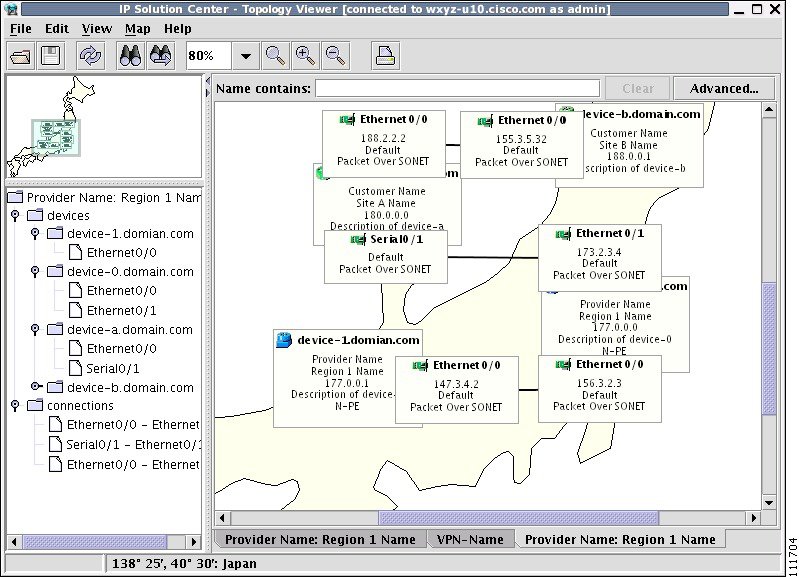
Adding New Maps
You might want to add your own maps to the selection of maps available to the topology application. This is done by saving maps in the root directory. To make this example more accessible, assume that you want to add a map of Toowong, a suburb of Brisbane, the capital of Queensland. The first step to do so is to obtain maps from a map vendor. All maps must be in the ESRI shape file format (as explained at the web site: http://www.esri.com). In addition, a data file might accompany each shape file. Data files contain information about objects whose shapes are contained within the shape file. Let us assume that the vendor provided four files:
•![]() toowong_city.shp
toowong_city.shp
•![]() toowong_city.dbf
toowong_city.dbf
•![]() toowong_street.shp
toowong_street.shp
•![]() toowong_street.dbf
toowong_street.dbf
Then assume you want to create a map file that informs the topology application about layers of the map. In this case, you have two layers: a city and a street layer. The map file, say, Toowong.map, would thus have the following contents:
toowong_city
toowong_street
It lists all layers that create a map of Toowong. The order is important, as the first file forms the background layer, with other layers placed on top of the preceding layers.
Having obtained shape and data files and having written the map file, decide on its location. As mentioned, Toowong is a suburb of Brisbane, located in Queensland, Australia. All map files must be located in or under the $PRIMEF_HOME/resources/webserver/tomcat/webapps/ipsc-maps/data directory. Since by default this directory contains a directory called Oceania intended for all maps from that region, simply create a path Australia/Queensland/Brisbane under the directory Oceania. Next, place all five files in this location. After this is done, the map is automatically accessible to the topology viewer.
 Feedback