Overview
These tutorials take you through the WAE Design GUI in a structured way so that you quickly get an overview of the user interface, including the basics of failure simulations.
-
Getting Started with WAE Design—Introduces you to the GUI, explains how to use the controls and menus, and shows you the basics of how to modify simulated traffic (demands).
-
Getting Started with Simulation Analysis—Demonstrates how to generate failure scenarios and how to examine your network for component failure vulnerabilities.
Getting Started with WAE Design
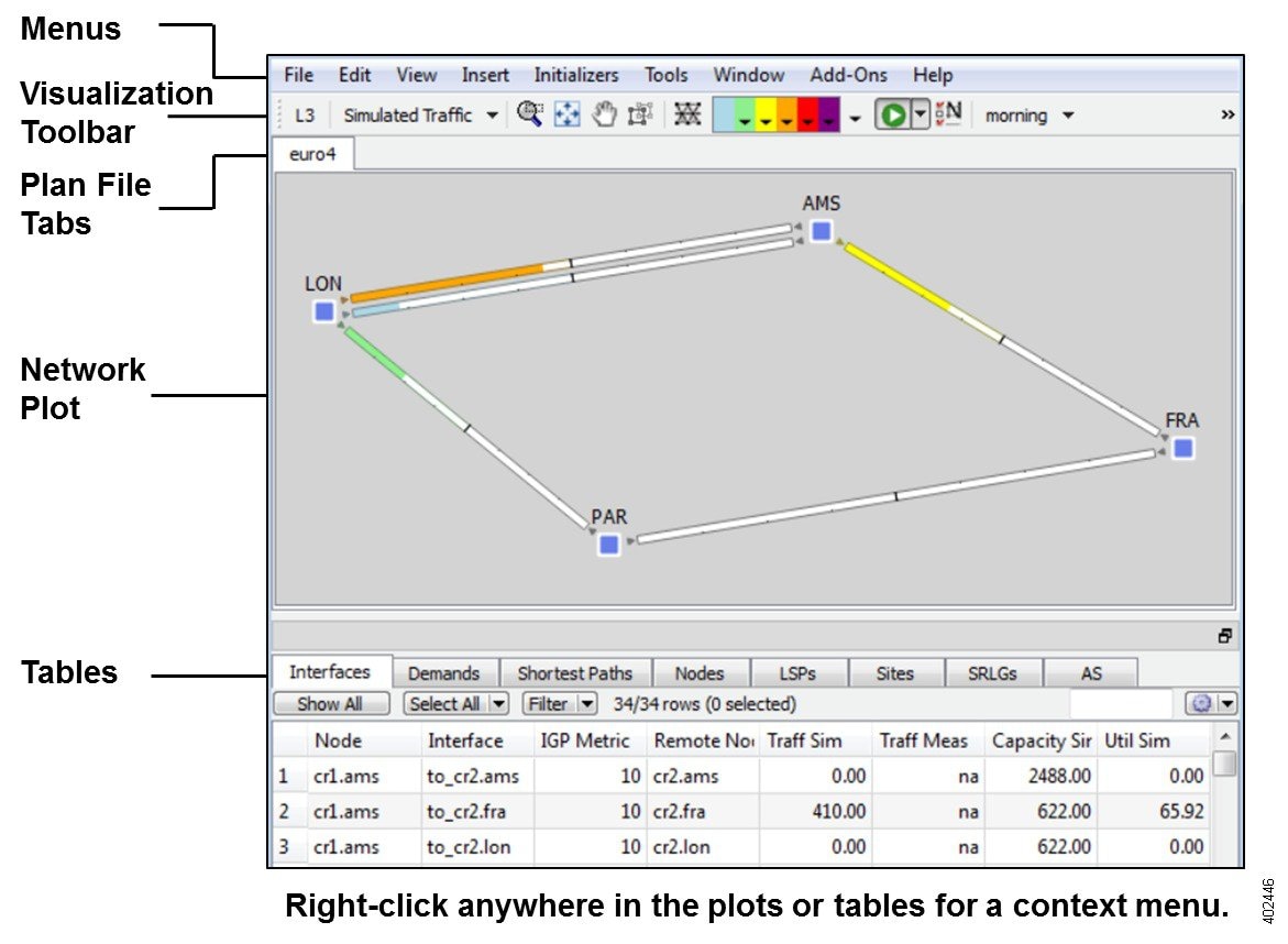
The WAE Design GUI operates on plan files, or plans, that contain the components of information that display the network. In this tutorial, you use sample plan files that come with the WAE Design application. Topics include:
-
WAE Design GUI display and behavior, including network plot, toolbars, tables, selection methods, and shortcuts.
-
Customizing displays for circuit capacities and traffic utilizations.
-
Traffic demands, which are the foundation for network modeling and simulation in WAE Design.
WAE Design works on both measured and simulated traffic. Traffic is simulated through demands (which are explained in Simulate Traffic Using Demands). Unless otherwise noted, the instructions and diagrams are for simulated traffic.
 Note |
This tutorial references $CARIDEN_HOME, which is the directory in which the Cisco WAE executables and binaries are installed. On Linux, the default $CARIDEN_HOME is /opt/cariden/software/mate/current, where /opt/cariden is the default installation directory. |
Launch WAE Design and Open a Plan File
To view the network topology and perform WAE Design operations, you must open a plan file. To use WAE Design effectively, it is helpful to understand the main GUI components.
Task: Launch WAE Design, open a plan file, and develop a basic understanding of the GUI.
Procedure
| Step 1 |
Double-click the wae_design icon in the $CARIDEN_HOME directory, which is the directory in which WAE Design is installed. |
| Step 2 |
If a license message is displayed, click OK to continue. (You don't need a license to use the sample plans.) |
| Step 3 |
Choose . |
| Step 4 |
Browse to $CARIDEN_HOME/samples and open the euro4.txt file, which is a sample European network. |
| Step 5 |
Locate each of the following GUI components:
 |
| Step 6 |
If continuing with these tutorials, keep this plan open for the next task. If stopping here, choose to close the file without saving it. |
View Network, Site, and Interface Plots
Upon opening the plan file used in this tutorial, the network plot shows sites (square icons) that appear to be connected by circuits, though they actually connect to nodes (routers) within each site. The nodes within the sites are connected with intrasite circuits. Each circuit consists of two interfaces that are delineated by the line in the middle of the circuit.
Note that sites can also contain other sites, and nodes do not have to be contained within sites.
Task: View network, site, and interface plots.
Procedure
| Step 1 |
If the euro4.txt file is not open, choose . Browse to $CARIDEN_HOME/samples and open the euro4.txt file. |
| Step 2 |
In the network plot, notice the four sites. These are connected by 622 Mbps (OC12/STM4) circuits. LON and AMS are connected by two such circuits. This information is listed in the Capacity Sim column of the Interfaces table. 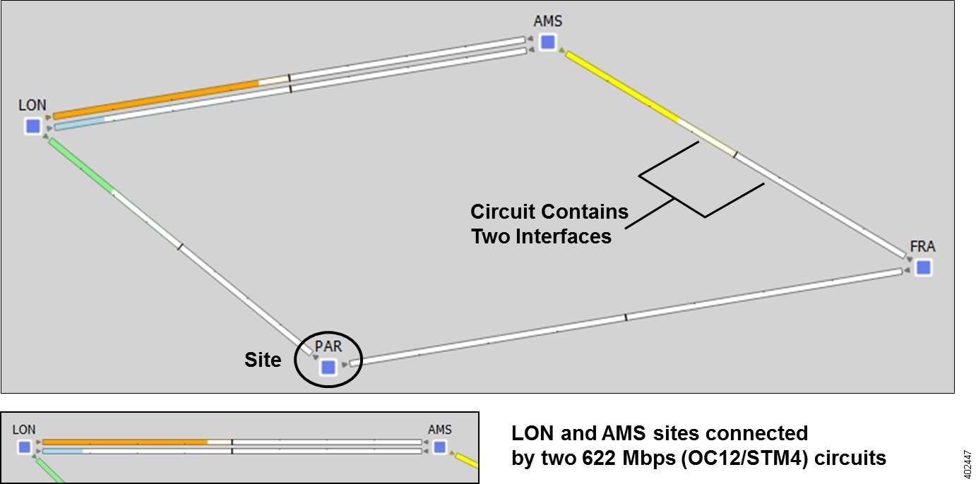 |
| Step 3 |
Open a site plot.
|
| Step 4 |
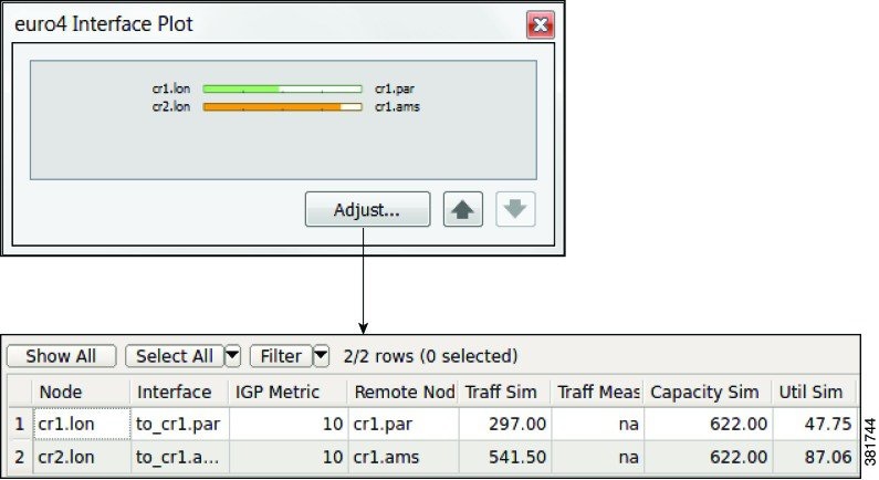
Open an interface plot. 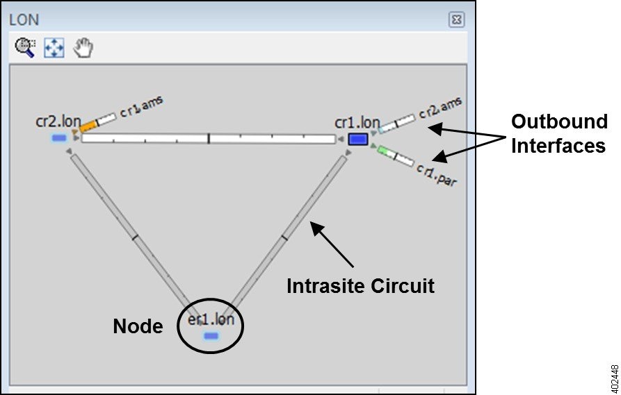
 |
| Step 5 |
If continuing with these tutorials, keep this plan open for the next task. If stopping here, choose to close the file without saving it. |
Work with Tables and Object Selections
This section familiarizes you with the basic dynamics between tables and objects, such as nodes, sites, circuits, interfaces, and ports. When you select an object in a table, it is automatically selected in the network plot. Conversely, whatever you select in the network plot is selected in the tables.
Task: Show different tables and select objects. Each time you make a selection, observe what happens in the tables and in the network plot to see their relationships.
Procedure
| Step 1 |
If euro4.txt file is not open, choose . Browse to $CARIDEN_HOME/samples and open the euro4.txt file. |
| Step 2 |
Notice that the Interfaces tab is selected. Click the Sites tab to show the Sites table. |
| Step 3 |
In the network plot, click various sites, and each time notice the blue highlight in the left column of the Sites table. Also notice that each time you select a new site, the other is no longer selected. This is because selecting an individual object deselects all others. |
| Step 4 |
Show the Circuits table, which is not in the default table tabs.
|
| Step 5 |
In the Circuits table, select the PAR-LON circuit. Press and hold Ctrl (Cmd on a Mac) while clicking the AMS-FRA circuit. Notice that both rows are highlighted as are the corresponding circuits in the network plot. This selects four interfaces (two interfaces per circuit). To verify these selections, in the Circuits table right-click either of the two selected circuits, and choose Filter to Interfaces. The Interfaces table shows the four interfaces that are selected in the network plot. |
| Step 6 |
In the Interfaces table, click Show All. |
| Step 7 |
Click the top row of the Interfaces table. Press and hold Shift while clicking the fourth row. All four interfaces are selected both in the table and in the plot. Two of these interfaces are intrasite as indicated by the small square on top of the AMS site.
 |
| Step 8 |
If continuing with these tutorials, keep this plan open for the next task. If stopping here, choose to close the file without saving it. |
Change Circuit Capacity Width
Circuits are drawn to show the relationship of their capacity to their utilization. By default, the width of the circuit is proportional to the capacity, down to a predefined minimum width, and the interfaces appear without explanatory text. The Plot Options icon opens a dialog box where you can change the relationship between width and capacity, and control the minimum width and rate at which the width changes for different capacities.
Task: Change the relationship between circuits’ width and their capacity.
Procedure
| Step 1 |
If the euro4.txt file is not open, choose . Browse to $CARIDEN_HOME/samples and open the euro4.txt file. |
| Step 2 |
Click the Plot Options icon in the top right of the visualization toolbar; the Plot Options dialog box opens. 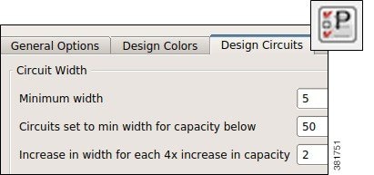 |
| Step 3 |
In the Design Circuits tab, change the value in the “Circuits set to min width for capacity below” field from 580 to 50, and click OK. |
| Step 4 |
Notice that all circuits are wider than the minimum now because their capacities all exceed 50 Mbps. 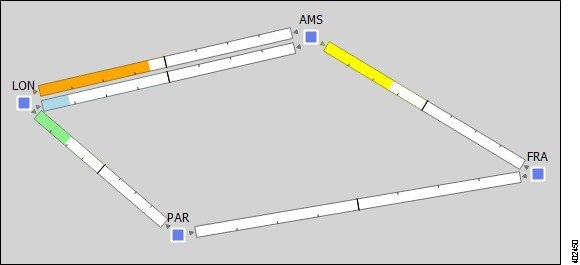 |
| Step 5 |
Double-click the LON site to open its site plot. Notice that some circuits show at the minimum width with no fill color; this is because these circuits do not have a specified capacity. |
| Step 6 |
Reopen the Plot Options dialog box, change the setting back to the default of 580, and click OK. |
| Step 7 |
If continuing with these tutorials, keep this plan open for the next task. If stopping here, choose to close the file without saving it. |
Determine Traffic Utilization
WAE Design shows either measured network traffic or simulated traffic, depending on the view. The color fill of an interface shows the bandwidth utilization for traffic leaving that interface in proportion to the interface capacity. That is, it shows the traffic utilization.
The exact utilization of any circuit is listed in the tables where all quantitative parameters of the network are available. You can customize the colors and thresholds from the Utilization Color menu.
Task: Determine the traffic utilization threshold using color fills, Util Sim column, and textual representations.
Procedure
| Step 1 |
If euro4.txt file is not open, choose . Browse to $CARIDEN_HOME/samples and open the euro4.txt file. |
| Step 2 |
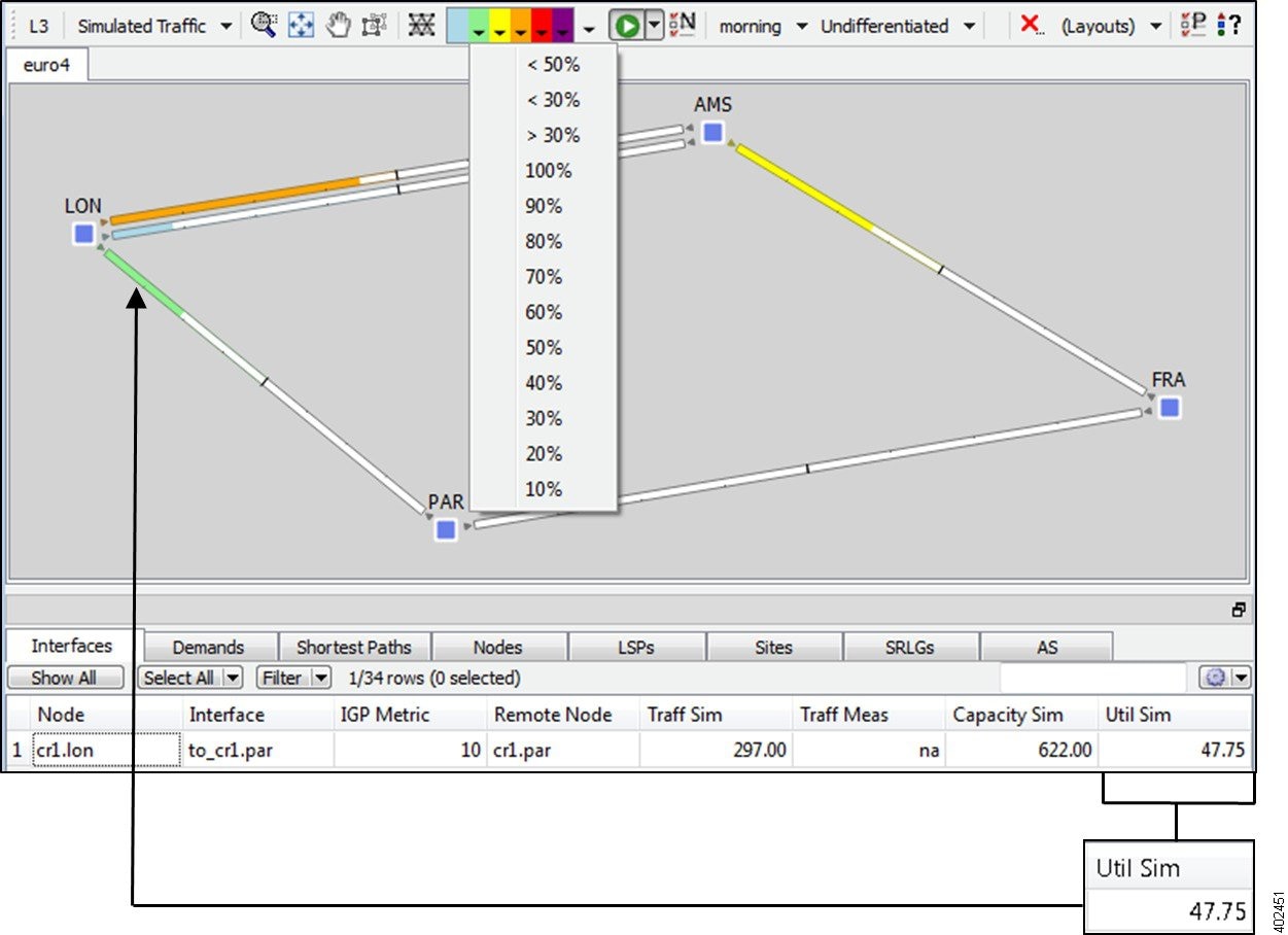
Click the green drop-down arrow in the Utilization Color menu. The range indicates that if an interface is green, its traffic utilization is between 30-50%. 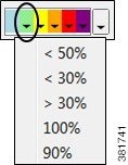 |
| Step 3 |
In the network plot, click the green part of the circuit between LON and PAR. Right-click this interface and choose Filter to Selection. The Interfaces table opens and shows only this interface. |
| Step 4 |
Note that the Util Sim (simulated) column shows a utilization of 47.75% for this interface, which is between the 30-50% level denoted by green as shown in the Utilization Color drop-down menu. The interface is filled with green that extends to fill almost half of this interface. The other half of the circuit displays the traffic utilization for the reverse direction, which is 0% for this interface. |
| Step 5 |
In the Interfaces table, click Show All. |
| Step 6 |
Identify the percentages by displaying them on all interfaces.
 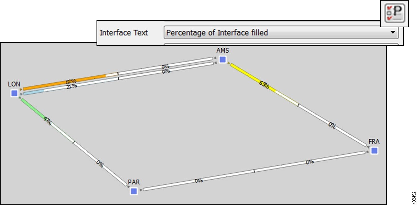 |
| Step 7 |
If continuing with these tutorials, keep this plan open for the next task. If stopping here, choose to close the file without saving it. |
Most Highly Utilized Interface
There are two ways to identify the most utilized interfaces, which is useful when analyzing large, complex networks.
Task: Determine the most highly utilized interfaces in the network using each of the following methods.
Method: Sort Util Sim Column
Procedure
| Step 1 |
If euro4.txt file is not open, choose . Browse to $CARIDEN_HOME/samples and open the euro4.txt file. |
| Step 2 |
In the Interfaces table, click the Util Sim column heading to sort the interfaces by descending order. Click it two more times; the column sort toggles between ascending and descending order. |
| Step 3 |
Notice that the most utilized interface is at 87.06% of capacity, which is the top row. Click this top row. The interface highlighted in the plot is the most highly utilized interface. |
| Step 4 |
Use the down arrow to move down row by row, each time finding the next most highly utilized interface. Each selection is highlighted in the plot and its exact utilization value is visible in the Util Sim column. |
| Step 5 |
Click in an empty plot area to deselect the interfaces. |
Method: Select Max Value in Utilization Color Menu
Procedure
| Step 1 |
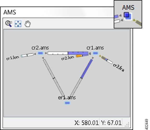
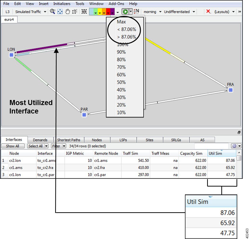
Click the purple drop-down arrow in the Utilization Color menu to see that the maximum utilization value is 100%. Choose Max. This resets the maximum threshold percentage to the most highly utilized interface, which color fills that interface, cr2.lon-cr1.ams, to purple. 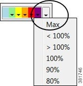 |
| Step 2 |
Click the purple drop-down arrow again to see that maximum is now 87.06%. Verify this by reading its Util Sim value in the Interfaces table, which is also 87.06%. |
| Step 3 |
Click the purple drop-down arrow again and choose < 87.06%. This highlights the second most highly utilized interface, which is cr1.ams-cr2.fra. |
| Step 4 |
Set the maximum utilization back to 100% by restoring the system default colors:
 |
| Step 5 |
If continuing with these tutorials, keep this plan open for the next task. If stopping here, choose to close the file without saving it. |
Simulate Traffic Using Demands
Several WAE Design tables have columns that identify how much traffic is being carried or what percentage of the capacity is being utilized. For example, the Interfaces table has a Util Sim column that reflects simulated traffic utilization. The two basic inputs to the simulation are the network configuration itself and a set of traffic demands. A demand is a request for a specified amount of traffic to be sent from one node, the source, to another node, the destination. The routes taken are based on traffic, topology, network health, as well as the protocols used.
Task: Determine which service classes are associated with demands, read demand traffic and latency, and identify demands route in the network plot.
Procedure
| Step 1 |
Choose . Browse to $CARIDEN_HOME/samples and open the euro4.txt file. |
| Step 2 |
Click the Demands tab to show the Demands table. Notice that this network contains only six demands, all from the er1.lon edge node in the LON site to the edge notes in other sites. |
| Step 3 |
Show the Service Class column:
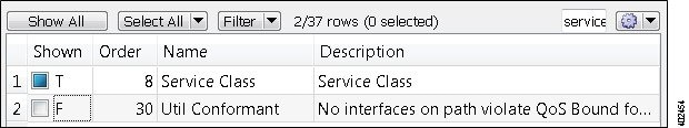 |
| Step 4 |
Click the Service Class column heading to sort demands by service class, noting that half the demands represent Internet traffic and half represent voice traffic. |
| Step 5 |
Read the Traffic column values to determine how much traffic each demand is attempting to route. |
| Step 6 |
Determine the sum of the delays for all the interfaces on the longest path taken by each demand:
|
| Step 7 |
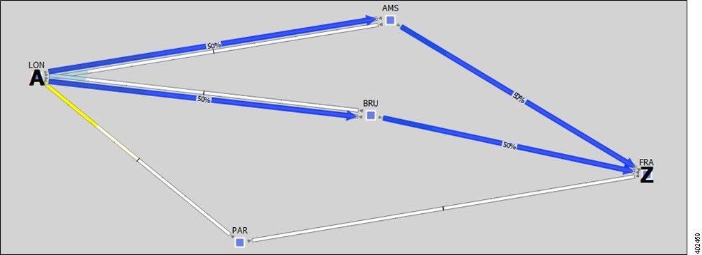
In the Demands table, click the demand from er1.lon to er1.par. The network plot shows this demand from LON to PAR sites using a blue arrow to show the route, an A to show the source, and a Z to show the destination. 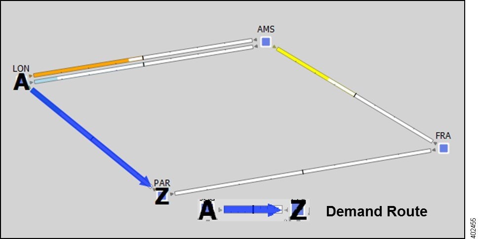 |
| Step 8 |
Use the up and down arrow keys to move from row to row in the Demands table, highlighting each demand and showing its routing in the network. Notice the er1.lon to er1.ams demand takes two equal-cost multipath (ECMP) routes along two parallel circuits. Two blue lines show 50% of the traffic flowing through each of these circuits. |
| Step 9 |
Right-click the er1.lon to er1.ams demand and choose Plot Demands. This view shows the details of the demand route. |
| Step 10 |
Close the demands plot. |
| Step 11 |
Click in an empty plot area to deselect the demand. 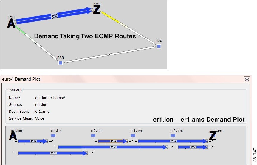 |
| Step 12 |
If continuing with these tutorials, keep this plan open for the next task. If stopping here, choose to close the file without saving it. |
Modify Demand Traffic
You can modify demand traffic to determine the effects such changes in traffic have on the network. These modifications can be applied to regions or sites, or they can apply uniformly over the network, such as in the following task.
For instance, you might increase demand traffic to plan for future traffic growth by simulating an overall traffic growth trend. Another example use might be to determine the network impact of an anticipated increase in sales of a particular service, such as video on demand.
Task: Simulate an increase in voice traffic by 50%.
Procedure
| Step 1 |
Choose . Browse to $CARIDEN_HOME/samples and open the euro4.txt file. |
| Step 2 |
Locate all voice demands by filtering:
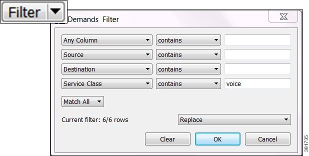 |
| Step 3 |
Increase the demand traffic for all voice demands by 50%:
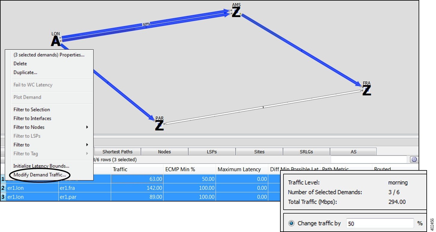 |
| Step 4 |
Click anywhere in the empty plot area to remove the demand selections. |
| Step 5 |
Read the values in the Traffic column and note they have increased by 50% to 94.5, 133.5, and 213 Mbps. The plot shows that modifying this traffic created severe congestion between LON and AMS as noted by the purple color fill. Compare, for example, the color of interfaces between LON and AMS to those prior to the simulated traffic increase. 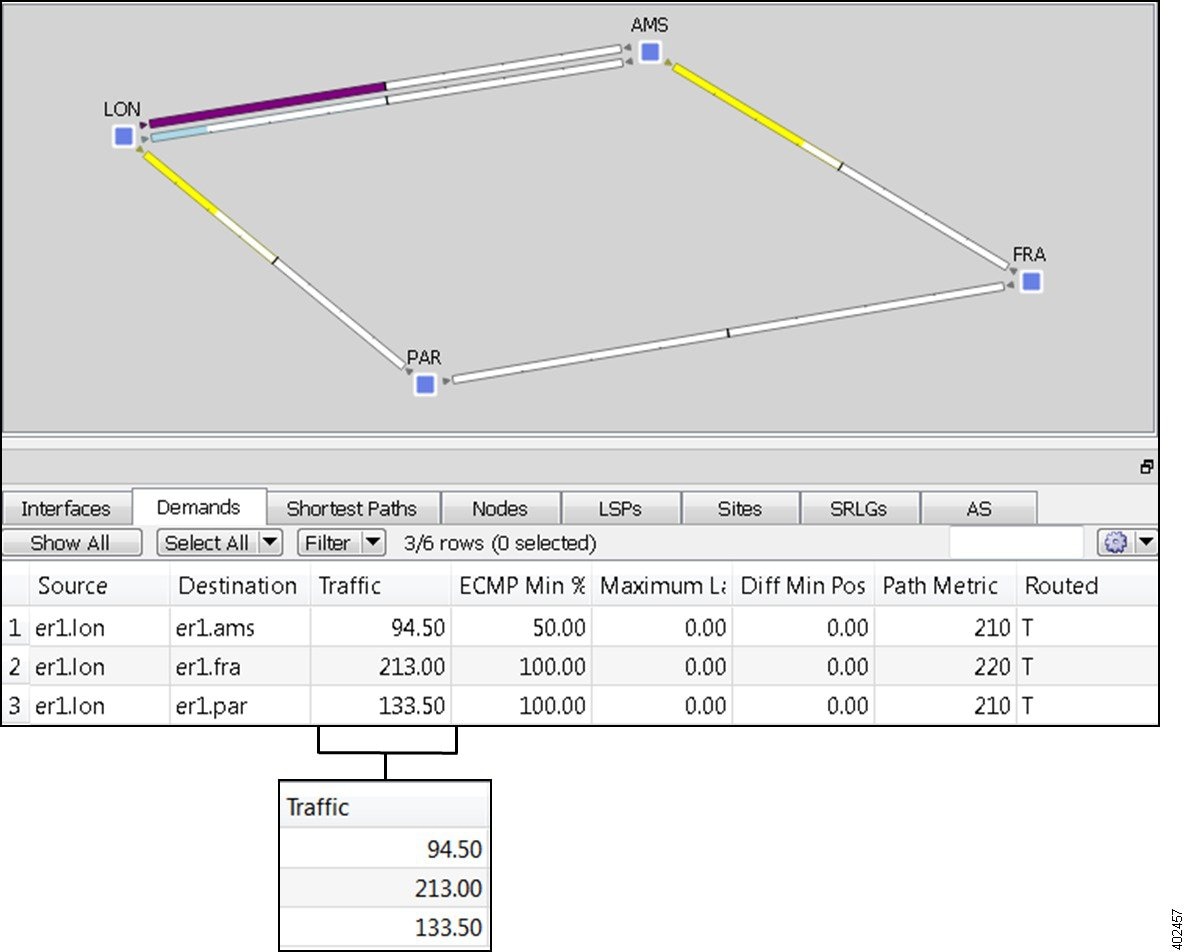 |
| Step 6 |
Choose to close the file without saving it. |
Edit Topology
WAE Design tools let you edit the network topology so that you can add, delete, and move objects. Some tools, such as the duplication function, greatly simplify the redesign of a complex network.
Once topology changes are made, demands are rerouted, showing the resulting utilization changes in the new network.
Task: Create a new site by duplicating an existing one, place it in its geographically correct location, and observe how traffic is rerouted as a result of the topology change.
Procedure
| Step 1 |
Choose . Browse to $CARIDEN_HOME/samples and open the euro4.txt file. |
| Step 2 |
Because you are determining the effect of adding a site, view the demand route before editing the topology:
|
| Step 3 |
Create a BRU site by duplicating the AMS site:
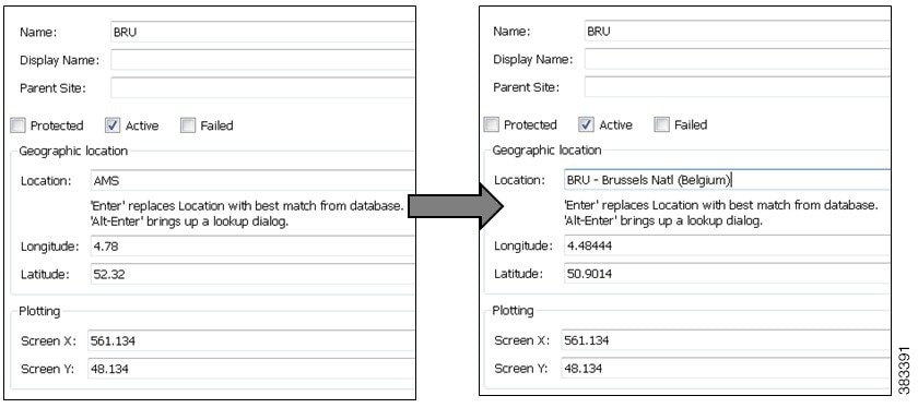 |
| Step 4 |
Place the site on the plot using its newly updated geographic location:
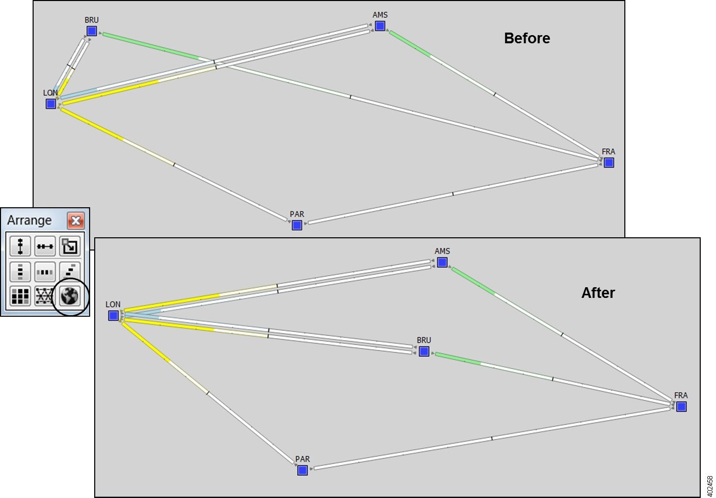 |
| Step 5 |
Observe the effect of adding this new site as it reroutes the er1.lon-er1.fra demand:
 |
| Step 6 |
Choose to close the file without saving it. |
Getting Started with Simulation Analysis
WAE Design Simulation lets you perform failure analysis, which can be useful in long-term planning and short-term preparation. For example, WAE Design simulates reroutings and changes in traffic utilization under individual failure events, as well as across multiple failure scenarios that cause worst-case utilizations. This tutorial guides you through a sample of these failure analysis tasks.
For detailed information about simulating and analyzing failures, see the Cisco WAE Design User Guide.
Note |
This tutorial references $CARIDEN_HOME, which is the directory in which the Cisco WAE executables and binaries are installed. On Linux, the default $CARIDEN_HOME is /opt/cariden/software/mate/current, where /opt/cariden is the default installation directory. |
Failures
One of the most useful features of WAE Design is its ability to show network behavior when objects fail. For example, your network might show utilizations are well under 100% under normal operation. But what happens under failure?
Task: Determine the effects on the network if a single circuit fails.
Procedure
| Step 1 |
Choose . Browse to $CARIDEN_HOME/samples and open the us_wan.txt file. |
| Step 2 |
Notice all traffic utilization is under 100%. You can tell this because none of the interfaces are purple, which by default means over 100% utilized. Also, the Util Sim column in the Interfaces table shows no values over 100. |
| Step 3 |
Right-click the wdc side of the wdc-nyc circuit (cr2.wdc-cr1.nyc interface) and choose . |
| Step 4 |
Click the er1.atl to er1.bos (first) demand to see its route. The solid blue arrow shows the demand path. |
| Step 5 |
Right-click the wdc-nyc circuit and choose Fail. The red cross on the circuit indicates a failure. Notice the difference in traffic utilization colors in the plot. For example, the kcy-wdc circuit is now congested. |
| Step 6 |
Notice how the demand has been rerouted. The dashed line shows the current demand path under failure. Continue clicking different demands to see how they are rerouted. |
| Step 7 |
To restore the failed circuit, right-click it and choose Recover. |
| Step 8 |
Click anywhere in an empty plot area to deselect the demand. 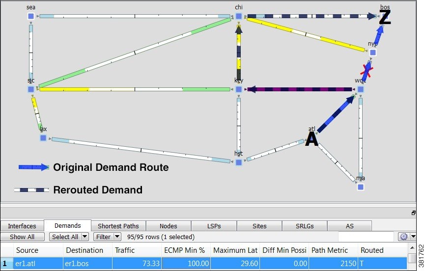 |
| Step 9 |
If continuing with this tutorial, keep this plan open for the next task. If stopping here, choose to close the file without saving it. |
SRLG Failures
A shared-risk link group (SRLG) is a group of objects that would likely fail due to a common cause. In a production network, the most common type of SRLG is one that contains circuits that share a common fiber. If the fiber fails, all circuits fail.
Several WAE Design tools let you simulate SRLG behavior; for example, Simulation Analysis can provide a worst-case analysis of utilizations over SRLG failures. Metric Optimization can optimize routing over failure scenarios that include SRLGs.
Task: Create an SRLG and fail it to observe the consequences to network traffic.
Procedure
| Step 1 |
If the us_wan.txt file is not open, choose . Browse to $CARIDEN_HOME/samples and open the us_wan.txt file. |
| Step 2 |
Create an SRLG: 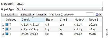 |
| Step 3 |
Verify the SRLG1 is in the SRLGs table. |
| Step 4 |
Right-click SRLG1 and choose Fail. The followng figure shows the circuits that belong to the failed SRLG and the resulting severe congestion. The red crosses with white fill mean these circuits are still active, but are not operational because of other failures. |
| Step 5 |
To recover the SRLG, right-click in an empty plot area and choose Recover. 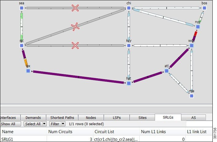 |
| Step 6 |
Keep this plan open and continue to the next task. If you are stopping here and plan to continue later, choose and save the plan file to a different location. |
Simulation Analysis
The Simulation Analysis tool simulates network behavior across multiple failure scenarios, multiple traffic levels, and over multiple service classes.
Task: Determine the network repercussions of failing single circuits and SRLGs to their worst-case utilizations.
Procedure
| Step 1 |
This task uses the us_wan.txt file that contains the SRLG created and saved in the preceding section. If it is not open, choose and browse to its location to open it. |
| Step 2 |
Choose and choose the failure scenarios over which to run the analysis. |
| Step 3 |
Check the Circuits and SRLGs check boxes. |
| Step 4 |
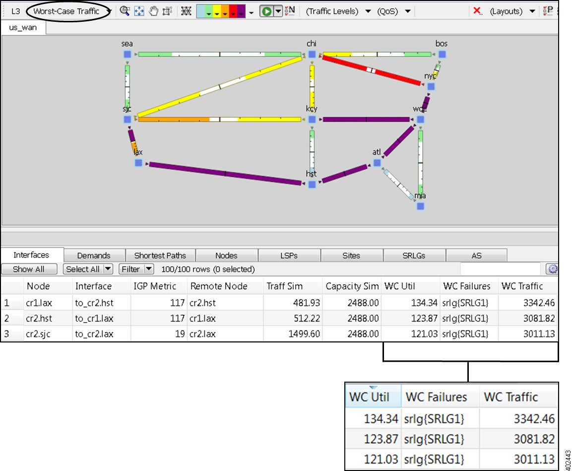
Retain all defaults and click OK. By default, the tool records up to 10 failure scenarios per interface that cause the worst-case utilization. WAE Design now performs a simulation for each possible circuit failure and each SRLG failure in the network, and calculates the utilization for these failure scenarios. The plot shows the resulting congestion in the Worst-Case Traffic view. |
| Step 5 |
Find the interface. |
| Step 6 |
When all simulations are complete, a report displays the results.
 |
| Step 7 |
Keep this plan open for the next task. |
Worst-Case Failure Analysis: Example 1
In the Worst-Case Traffic view the interfaces are colored based on their worst-case utilizations over all the scenarios specified for the simulation analysis. This view is useful to see which circuits would become congested under different failure scenarios, and to discover the cause of their worst-case loading on a circuit-by-circuit basis.
To better understand the meaning of the plot, imagine that for each simulation case (here, each possible circuit or SRLG failure) a transparent plot was generated. After all scenarios are run, the plots are placed on top of one another and the worst-case utilization for all circuits is displayed in the plot. It is likely that different failure scenarios produce the worst-case utilization for different circuits.
Task: Determine which interface had the worst-case traffic utilization under this failure scenario, and determine the failures causing it.
Procedure
| Step 1 |
Continue using the us_wan.txt file on which you created an SRLG and ran a worst-case simulation analysis. If you are reopening the file, it must contain the SRLG, and you must perform the previous task that runs a simulation analysis to fail circuits and SRLGs to their worst case. |
| Step 2 |
To find the interface with the worst-case utilization over all failure scenarios calculated for this simulation analysis, click the WC Util column in the Interfaces table to toggle it to the highest-to-lowest sort order. The cr1.lax to cr2.hst interface has the most with 134.34%. |
| Step 3 |
Look at the WC Failures column to note which failures cause the worst-case utilization on this interface. Here, the SRLG1 failure is the culprit. |
| Step 4 |
Keep this plan open for the next task. |
Worst-Case Failure Analysis: Example 2
Task: View the failure scenarios that cause the worst-case utilization for the cr1.nyc to cr2.wdc interface and simulate one to determine how the network would react to this failure.
Procedure
| Step 1 |
Continue using the us_wan.txt file on which you ran a worst-case simulation analysis across circuits and SRLGs. |
| Step 2 |
In the Interfaces table, right-click the interface going from node cr1.nyc to cr2.wdc and choose Fail to WC. The dialog box that opens lists two failures that would cause worst-case utilization on this interface. Select the first one, ct{cr1.kcy|{to_cr1.sjc}|cr1.sjc{to_cr1.kcy}}, and click OK. The plot now shows the effects of this failure scenario, and therefore changes to a Simulated Traffic view. 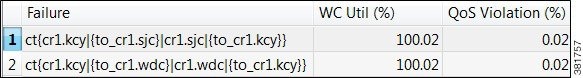 |
| Step 3 |
To recover the failed circuit, right-click in an empty plot area and choose Recover. 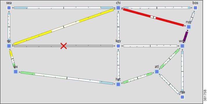 |
| Step 4 |
Keep this plan open for the next task. |
Worst-Case Failure Analysis: Example 3
Task: View the worst-case information over a subset of the failure set without rerunning the analysis.
Procedure
| Step 1 |
Continue using the us_wan.txt file on which you previously ran a worst-case simulation analysis across circuits and SRLGs. |
| Step 2 |
From the Network Plot View drop-down list, choose Worst-Case Traffic. |
| Step 3 |
Click the red X in the top right of the visualization toolbar. A dialog box lets you select a subset of the simulated failure scenarios to view. |
| Step 4 |
Uncheck the SRLGs check box and click OK. The network plot changes to reflect utilizations over circuit failures only. The WC Util column in the Interfaces table changes to show maximum utilizations over circuit failures only. The WC Failures column shows only circuit failures resulting in these utilizations. 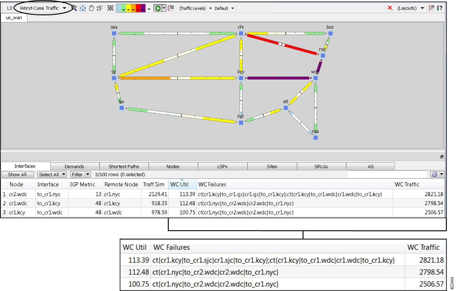 |
| Step 5 |
Keep this plan open for the next task. |
Failure Impact Analysis
The Failure Impact view colors each node and circuit to the maximum utilization level that would be caused elsewhere in the network if it were to fail. For example, by default red means a circuit is between 90 to 100% utilized. A circuit that is red in the Failure Impact view means that if that circuit were to fail, it would cause other nodes or circuits to go to 90-100% utilization. This Failure Impact analysis is automatically calculated each time you run Simulation Analysis.
Task: View the Failure Impact to note the impact circuit failures would have on the network.
Procedure
| Step 1 |
Continue using the us_wan.txt file on which you ran a simulation analysis in the previous task on circuits only. If you are reopening the file, you must run a worst-case simulation analysis that fails only circuits. |
| Step 2 |
From the Network Plot View drop-down list, choose Failure Impact. |
| Step 3 |
Show the Failure Impact row in the Interfaces table:
|
| Step 4 |
Study the plot to determine potential problems for the network should a circuit fail. 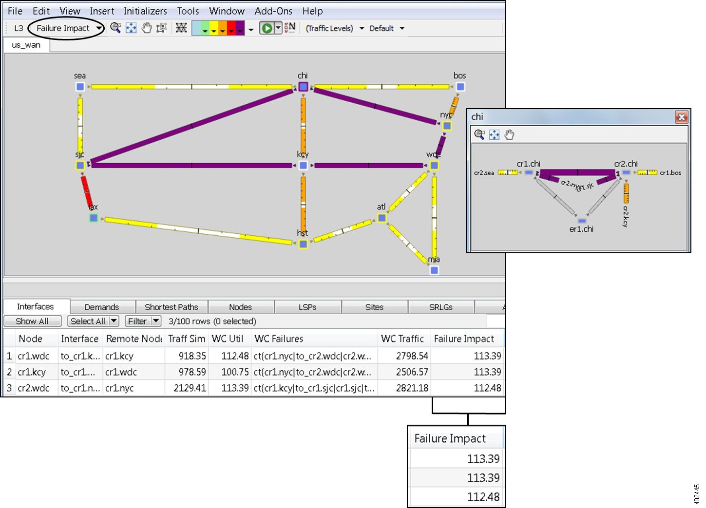 |
| Step 5 |
Choose to close the file without saving it. |
 Feedback